bistaticReceiver
Description
bistaticReceiver creates a bistatic receiver object. Bistatic radar
      systems have separate transmitter and receiver elements that are not co-located. To create a
      bistatic radar that supports synchronous, asynchronous, and multiple transmitter and receiver
      pairs, use bistaticTransmitter in conjunction with
      bistaticReceiver.
Receive signals from the bistatic receiver by calling the receive object
      function. Optionally collect and coherently combine signals using the collect object
      function prior to calling receive. The nextTime object
      function returns the start time of the next receive window.
For a typical bistatic workflow, construct the bistatic transmitter using
        bistaticTransmitter and construct the bistatic receiver using
        bistaticReceiver. Then, transmit the waveform by calling
        transmit on the bistatic transmitter. Finally, call receive on the
      bistatic receiver to receive the propagated signal returned by transmit.
      For a more advanced workflow that supports multiple transmitters and parallelization, call
        collect on the
      bistatic receiver to coherently combine the transmitted signal returned by
        transmit prior to calling receive. See Transmit, Collect, and Receive Timing Visualization for more information on
      simulation timing and using information provided by nextTime.
Creation
Description
RX = bistaticReceiverRX, that is used to receive
          signals transmitted by bistaticTransmitter. Call
            receive on RX to generate samples from
          transmitted signals collected by the receive antenna and propagated through the
          receiver.
RX = bistaticReceiver(PropertyName=Value)RX, with each specified
            PropertyName set to the corresponding Value.
          You can specify additional pairs of arguments in any order as
            PropertyName1=Value1,...,PropertyNameN=ValueN.
Properties
Radar receiver, specified as a phased.Receiver
            System object™. The default receiver is a phased.Receiver system object
            with default values.
Radar receive antenna, specified as a phased.Collector
            System object. The default radiator is a phased.Collector system object
            with default values. The Polarization property of the
              phased.Collector must be set to "None".
              Polarization properties "Dual" and
              "Combined" are not supported.
Receive window duration, specified as a positive scalar in units of seconds. The
            receive window duration is the length of the receive window. A new receive window starts
            after the WindowDuration elapses.
              WindowDuration times SampleRate must be
            equal to an integer. After the property validation process, a warning will be given and
            the WindowDuration will be adjusted to the closest number that
            satisfies this conditions, if necessary. The default value is 0.0001 seconds.
Data Types: double
Receive window idle time, specified as a nonnegative scalar in units of seconds. The
            receive window idle time can be used to simulate times when the receiver is not active.
            If continuous receive is desired, set WindowIdleTime to 0. The
              WindowIdleTime times SampleRate must be
            equal to an integer. After the property validation process, a warning will be given and
            the WindowIdleTime will be adjusted to the closest number that
            satisfies this conditions, if necessary. The default value is 0 seconds.
Data Types: double
Source of the maximum collect buffer duration, specified as
              "Auto" or "Property". When
              MaxCollectDurationSource is set to "Auto", the
            collect buffer automatically grows to accommodate additional transmissions. When the
            value is set to "Property", the collect buffer has a fixed duration
            specified by the MaxCollectDuration property. Transmissions that
            are collected with delays that exceed the buffer duration are discarded. The default
            value is "Auto".
Data Types: string | char
Maximum duration of the collect buffer, specified as a non-negative scalar in units
            of seconds. The collect buffer duration determines the maximum duration beyond the end
            of the receive window that can be collected for the next receive window. Longer collect
            durations can prevent reflections with long propagation delays from being dropped
            between receive windows. The MaxCollectDuration times the
              SampleRate must be equal to an integer. After the property
            validation process, a warning will be given and the
              MaxCollectDuration will be adjusted to the closest number that
            satisfies this conditions, if necessary. The default value is 1 second.
Dependencies
To enable this property, set the MaxCollectDurationSource
              property to "Property". 
Data Types: double
Sample rate, specified as a positive scalar in units of hertz.
              SampleRate relates to the WindowDuration,
              WindowIdleTime, and MaxCollectDuration
            property. The default value is 1e6 (1 MHz).
Data Types: double
Initial receive time of the start of the first receive window, specified as a non-negative scalar in units of seconds. The default value is 0 seconds.
Data Types: double
This property is read-only.
SimulationTime indicates the current simulation time of the
            bistatic radar receiver, specified in units of seconds.
Data Types: double
Object Functions
Examples
This example shows how to create a bistatic scenario with two bistatic transmitters. The receiver is located between the transmitters and there is a target with a custom radar cross section. Transmit and collect pulses for four receive windows and plot the results.
Configure the bistatic transmitters. Use a pulse repetition frequencey of 1000 Hz.
prf = 1e3; wav = phased.LinearFMWaveform(PRF=prf,PulseWidth=0.2/prf); ant = phased.SincAntennaElement(Beamwidth=10); tx1 = bistaticTransmitter(Waveform=wav, ... Transmitter=phased.Transmitter(Gain=40), ... TransmitAntenna=phased.Radiator(Sensor=ant)); tx2 = clone(tx1); prf = 2e3; tx2.Waveform = phased.RectangularWaveform( ... PRF=prf,PulseWidth=0.2/prf); tx2.Transmitter.PeakPower = 2e3;
Configure the bistatic receiver.
rx = bistaticReceiver( ... ReceiveAntenna=phased.Collector(Sensor=ant), ... WindowDuration=0.0025); freq = tx1.TransmitAntenna.OperatingFrequency;
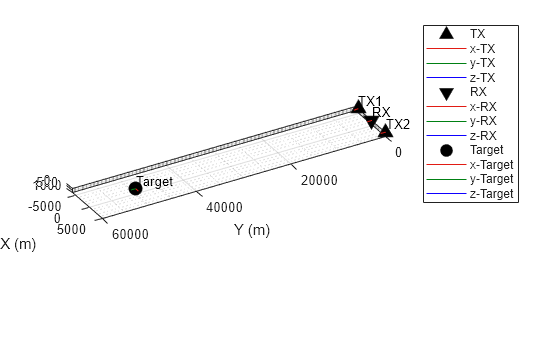
Create bistatic transmitter platforms spaced 10 km apart. Put the receiver platform between the two transmitters.  For this example, create the platforms in radarScenario. Define the platforms using platform.
scene = radarScenario(UpdateRate=prf); tx1Plat = platform(scene,Position=[-5e3 0 0], ... Orientation=rotz(85).'); tx2Plat = platform(scene,Position=[5e3 0 0], ... Orientation=rotz(95).'); rxPlat = platform(scene,Position=[0 0 0], ... Orientation=rotz(90).');
Place a stationary target platform down range and assign the target a radar cross section.
rcsSig  = rcsSignature(Pattern=20); 
tgtPlat = platform(scene,Position=[0 50e3 0], ...
        Signatures=rcsSig);Show platform locations and orientations.
tp = theaterPlot(Parent=axes(figure)); txPltr = orientationPlotter(tp,Marker="^", ... DisplayName="TX",LocalAxesLength=1e3); rxPltr = orientationPlotter(tp,Marker="v", ... DisplayName="RX",LocalAxesLength=1e3); tgtPltr = orientationPlotter(tp,Marker="o", ... DisplayName="Target",LocalAxesLength=1e3); poses = platformPoses(scene); plotOrientation(txPltr,[poses(1:2).Orientation], ... reshape([poses(1:2).Position],3,[]).',["TX1" "TX2"]); plotOrientation(rxPltr,poses(3).Orientation,poses(3).Position,"RX"); plotOrientation(tgtPltr,poses(4).Orientation,poses(4).Position,"Target");

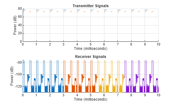
Transmit and collect pulses for four receive windows. First, update platform positions by calling advance on the scene. Then set up the for loop to iterate over the receive windows.  Next, get platform positions using platformPoses. Get the propogation paths for both transmitters using bistaticFeeSpacePath. Then, transmit the signal and collect pulses. Finally, receive the transmissions and plot the received signals.
tl = tiledlayout(figure,2,1); hAxes = [nexttile(tl) nexttile(tl)]; hold(hAxes,"on"); tx = {tx1 tx2}; advance(scene); for iRxWin = 0:4 [propSigs,propInfo] = collect(rx,scene.SimulationTime); t = min([nextTime(tx{1}) nextTime(tx{2})]); tEnd = nextTime(rx); while t <= tEnd % Get platform positions poses = platformPoses(scene); % Include target RCS signature on the pose tgtPose = poses(4); tgtPose.Signatures = {rcsSig}; for iTx = 1:2 % Calculate propogation paths proppaths = bistaticFreeSpacePath(freq, ... poses(iTx),poses(3),tgtPose); % Transmit [txSig,txInfo] = transmit(tx{iTx},proppaths,scene.SimulationTime); % Plot transmitted signal txTimes = (0:(size(txSig,1) - 1))*1/txInfo.SampleRate ... + txInfo.StartTime; plot(hAxes(1),txTimes*1e3,mag2db(max(abs(txSig),[],2)),SeriesIndex=iTx); % Collect transmitted pulses collectSigs = collect(rx,txSig,txInfo,proppaths); % Accumulate collected transmissions sz = max([size(propSigs);size(collectSigs)],[],1); propSigs = paddata(propSigs,sz) + paddata(collectSigs,sz); end t = min([nextTime(tx{1}) nextTime(tx{2})]); advance(scene); end % Receive collected transmissions [iq,rxInfo] = receive(rx,propSigs,propInfo); % Plot received transmissions rxTimes = (0:(size(iq,1) - 1))*1/rxInfo.SampleRate ... + rxInfo.StartTime; plot(hAxes(2),rxTimes*1e3,mag2db(abs(iq))); end
Label plots.
grid(hAxes,"on") title(hAxes(1),"Transmitter Signals") title(hAxes(2),"Receiver Signals") xlabel(hAxes,"Time (milliseconds)") ylabel(hAxes,"Power (dB)") ylim(hAxes(1),[0 80]); ylim(hAxes(2),[-130 -75]) xlim(hAxes(1),xlim(hAxes(2)))

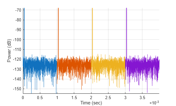
This example shows how to create a simple bistatic scenario with a moving target. Transmit and collect pulses until the completion of 1 receive window and plot the results.
Configure the bistatic transmitter and receiver. Use a pulse repetition frequency of 1000 Hz.
prf = 1e3; wav = phased.LinearFMWaveform(PRF=prf,PulseWidth=1e-5); ant = phased.SincAntennaElement(Beamwidth=10); tx = bistaticTransmitter(Waveform=wav, ... Transmitter=phased.Transmitter(Gain=20), ... TransmitAntenna=phased.Radiator(Sensor=ant)); rx = bistaticReceiver( ... ReceiveAntenna=phased.Collector(Sensor=ant), ... WindowDuration=0.005); freq = tx.TransmitAntenna.OperatingFrequency;
Create bistatic transmitter and bistatic receiver platforms spaced 10 km apart and add a target platform. Use radarScenario to crreate the platforms for this example.  Define the transmitter platform, receiver platform, and target platform using platform and give the target a trajectory.
scene = radarScenario(UpdateRate=prf); platform(scene,Position=[-5e3 0 0], ... Orientation=rotz(45).'); platform(scene,Position=[5e3 0 0], ... Orientation=rotz(135).'); traj = kinematicTrajectory( ... Position=8e3*[cosd(60) sind(60) 0],Velocity=[0 150 0]); tgtPlat= platform(scene,Trajectory=traj);
Create an empty plot.
hFig = figure; hAxes = axes(hFig);
Transmit and collect pulses for one receive window. First, update platform positions by calling advance on the scene and then get the platform positions using platformPoses. Next, get the propagation paths using bistaticFeeSpacePath. Then, transmit the signal and receive pulses. Finally, plot the received signals.
t = nextTime(tx); tEnd = nextTime(rx); while t < tEnd advance(scene); % Get platform positions poses = platformPoses(scene); % Calculate paths proppaths = bistaticFreeSpacePath(freq, ... poses(1),poses(2),poses(3)); % Transmit [txSig,txInfo] = transmit(tx,proppaths,t); % Receive pulses [iq,rxInfo] = receive(rx,txSig,txInfo,proppaths); t = nextTime(tx); % Plot received signals rxTimes = (0:(size(iq,1) - 1))*1/rxInfo.SampleRate ... + rxInfo.StartTime; plot(hAxes,rxTimes,mag2db(abs(sum(iq,2)))) hold(hAxes,'on') end
Label the plot.
grid(hAxes,'on') xlabel(hAxes,'Time (sec)') ylabel(hAxes,'Power (dB)') axis(hAxes,'tight')

More About
The current simulation time, the start of the leading edge of the next transmission time
        (returned by nextTime), and the start time of the next receive window
        (returned by nextTime) are important parameters in a bistatic
        simulation. In order to visualize how these simulation times relate to the transmitter pulse
        repetition interval (PRI), propagation delay, and receive window, consider a bistatic
        simulation in which there are two transmitters positioned along the base vertices of an
        isosceles triangle with the receiver positioned at the apex of the triangle. This symmetric
        geometry results in the same propagation delay for both transmitters.
For this simulation, the two transmitters have different PRIs and slightly different
        transmission start times. The first transmitter, TX1, has a PRI of
          PRI1. The second transmitter, TX2, has a PRI of
          PRI2. The signals from both transmitters will be collected over a
        duration of two PRI1 intervals. That is, the receive window for the
        receiver, RX, spans two PRI1 interval lengths. The
        figure below shows the current simulation time and the next transmission time returned by
          nextTime for each of five simulation steps that ends with the first
        receive window.
Simulation Step 1 — The signal transmitted from the antenna elements of TX1 is propagated to the receiver antenna elements and collected after the propagation delay.
- The current simulation time is the start of the transmit time for TX1. 
- TX2 will transmit in step 2 - Next TX2 Time is shown for reference. 
- TX1 will transmit again in step 3 - Next TX1 Time is shown for reference. 
- The returned collected signal is shifted forward in time by the propagation delay between the transmitter and the receiver. 
Simulation Step 2 — The signal transmitted from the antenna elements of TX2 is propagated to the receiver antenna elements and collected after the propagation delay.
- The current simulation time is the start of the transmit time for TX2, which corresponds to Next TX2 Time shown in the previous step. 
- TX1 will transmit in step 3 - Next TX1 Time is shown for reference. 
- TX2 will transmit again in step 4 - Next TX2 Time is shown for reference. 
- The returned collected signal is shifted forward in time by the propagation delay between the transmitter and the receiver. Signals that overlap in time are coherently combined at the receiver. 
Simulation Step 3 — The next signal transmitted from the antenna elements of TX1 is propagated to the receiver antenna elements and collected after the propagation delay.
- The current simulation time is the start of the transmit time for TX1, which corresponds to Next TX1 Time shown in the previous step. 
- TX2 will transmit in step 4 - Next TX2 Time is shown for reference. 
- TX1 will transmit again in step 5 - Next TX1 Time is shown for reference. 
- The returned collected signal is shifted forward in time by the propagation delay between the transmitter and the receiver. Signals that overlap in time are coherently combined at the receiver. 
Simulation Step 4 — The next signal transmitted from the antenna elements of TX2 is propagated to the receiver antenna elements and collected after the propagation delay.
- The current simulation time is the start of the transmit time for TX2, which corresponds to Next TX2 Time shown in the previous step. 
- TX1 will transmit in step 5 - Next TX1 Time is shown for reference. 
- TX2 will transmit again in step 6 (not shown) - Next TX2 Time is shown for reference. 
- The returned collected signal is shifted forward in time by the propagation delay between the transmitter and the receiver. Signals that overlap in time are coherently combined at the receiver. 
- The start of the first receive window, Next RX Time, is shown for reference. 
Simulation Step 5 — All signals previously collected from TX1 and TX2 are received. The next signal transmitted from the antenna elements of TX1 is propagated to the receiver antenna elements and collected after the propagation delay.
- The current simulation time is the start of the transmit time for TX1, which corresponds to Next TX1 Time shown in the previous step. The receive window also starts at the current simulation time, which corresponds to Next RX Time shown in the previous step. 
- TX2 will transmit in step 6 (not shown) - Next TX2 Time is shown for reference. 
- TX1 will transmit again in step 7 (not shown) - Next TX1 Time is shown for reference. 
- The returned collected signal is shifted forward in time by the propagation delay between the transmitter and the receiver. Signals that overlap in time are coherently combined at the receiver. 
- The receive window extends back in time for the length of the receive window to receive the previously collected transmitted signals. The next receive window will start after two PRI1 intervals (not shown). 
Version History
Introduced in R2025a
MATLAB Command
You clicked a link that corresponds to this MATLAB command:
Run the command by entering it in the MATLAB Command Window. Web browsers do not support MATLAB commands.
Seleccione un país/idioma
Seleccione un país/idioma para obtener contenido traducido, si está disponible, y ver eventos y ofertas de productos y servicios locales. Según su ubicación geográfica, recomendamos que seleccione: .
También puede seleccionar uno de estos países/idiomas:
Cómo obtener el mejor rendimiento
Seleccione China (en idioma chino o inglés) para obtener el mejor rendimiento. Los sitios web de otros países no están optimizados para ser accedidos desde su ubicación geográfica.
América
- América Latina (Español)
- Canada (English)
- United States (English)
Europa
- Belgium (English)
- Denmark (English)
- Deutschland (Deutsch)
- España (Español)
- Finland (English)
- France (Français)
- Ireland (English)
- Italia (Italiano)
- Luxembourg (English)
- Netherlands (English)
- Norway (English)
- Österreich (Deutsch)
- Portugal (English)
- Sweden (English)
- Switzerland
- United Kingdom (English)