Train DDPG Agent to Control Two-Thruster Sliding Vehicle

This example shows how to train a deep deterministic policy gradient (DDPG) agent to generate trajectories for a vehicle with two thrusters that slides without friction over a 2-D plane. The vehicle dynamics is modeled in Simulink®. For more information on DDPG agents, see Deep Deterministic Policy Gradient (DDPG) Agent.

For an example that shows how to use nonlinear model predictive control to solve the trajectory planning and control problems for a sliding vehicle, see Trajectory Optimization and Control of Sliding Robot Using Nonlinear MPC (Model Predictive Control Toolbox). For an example that shows how to train, validate, and test a deep neural network (DNN) that imitates the behavior of a nonlinear model predictive controller for a sliding vehicle, see Imitate Nonlinear MPC Controller for Sliding Robot.

Fix Random Number Stream for Reproducibility

The example code might involve computation of random numbers at several stages. Fixing the random number stream at the beginning of some sections in the example code preserves the random number sequence in the section every time you run it, which increases the likelihood of reproducing the results. For more information, see Results Reproducibility.

Fix the random number stream with seed 0 and random number algorithm Mersenne Twister. For more information on controlling the seed used for random number generation, see rng.

previousRngState = rng(0,"twister");

The output previousRngState is a structure that contains information about the previous state of the stream. You will restore the state at the end of the example.

Sliding Vehicle Model

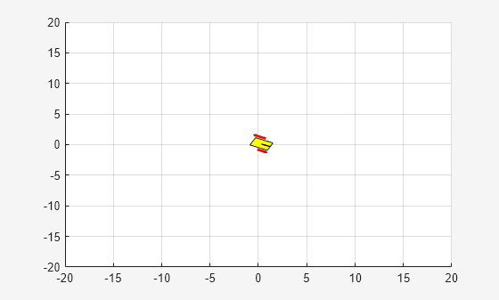
The reinforcement learning environment for this example is a sliding vehicle, implemented in Simulink®, with its initial condition randomized around a ring having a radius of 15 m. The orientation of the vehicle is also randomized. The vehicle has two thrusters mounted on the side of the body that are used to propel and steer the vehicle. The training goal is to drive the vehicle from its initial condition to the origin facing east.

Open the model.

mdl = "rlSlidingRobotEnv";
open_system(mdl)

Set the initial model state variables.

theta0 = 0;
x0 = -15;
y0 = 0;

Define the sample time Ts and the simulation duration Tf.

Ts = 0.4;
Tf = 30;

In this model:

• The goal orientation is 0 rad (vehicle facing east).

• The thrust from each actuator is bounded from -1 to 1 N

• The observations from the environment are the position, orientation (sine and cosine of orientation), velocity, and angular velocity of the vehicle.

• The reward $r_t$ provided at every time step is

$$r_1=10\left(\left({x_t}^2+{y_t}^2+{\theta }_t{}^2\right)<0.5\right)$$

$$r_2=-100\left(\left|x_t\right|\ge 20\left|\right|\left|y_t\right|\ge 20\right)$$

$$r_3=-\left(0.2{\left(R_{t-1}+L_{t-1}\right)}^2+0.3{\left(R_{t-1}-L_{t-1}\right)}^2+0.03{x_t}^2+0.03{y_t}^2+0.02{\theta }_t{}^2\right)$$

$$r_t=r_1+r_2+r_3$$

where:

• $x_t$ is the position of the vehicle along the x-axis.

• $y_t$ is the position of the vehicle along the y-axis.

• $\theta {}_t$ is the orientation of the vehicle.

• $L_{t-1}$ is the control effort from the left thruster.

• $R_{t-1}$ is the control effort from the right thruster.

• $r_1$ is the reward when the vehicle is close to the goal.

• $r_2$ is the penalty when the vehicle drives beyond 20 m in either the x or y direction. The simulation is terminated when $r_2<0$.

• $r_3$ is a QR penalty that penalizes distance from the goal and control effort.

For more information on this sliding vehicle model, see [1].

Create Closed Loop Simulink Model

To train an agent for the SlidingRobotEnv model, use the createIntegratedEnv function to automatically generate a Simulink model containing an RL Agent block that is ready for training.

integratedMdl = "IntegratedSlidingRobot";
[~,agentBlk,obsInfo,actInfo] = ...
    createIntegratedEnv(mdl,integratedMdl);

Actions and Observations

Before creating the environment object, specify names for the observation and action specifications, and bound the thrust actions between -1 and 1.

The observation vector for this environment is ${\left[\begin{array}{ccccccc}x& y& \underset{}{\overset{\dot{}}{x}}& \underset{}{\overset{\dot{}}{y}}& \sin \left(\theta \right)& \cos \left(\theta \right)& \underset{}{\overset{\dot{}}{\theta }}\end{array}\right]}^T$. Assign a name to the environment observation channel.

obsInfo.Name = "observations";

The action vector for this environment is ${\left[\begin{array}{cc}{T}_R& T_L\end{array}\right]}^T$. Assign a name, as well as upper and lower limits, to the environment action channel.

actInfo.Name = "thrusts";
actInfo.LowerLimit = -ones(prod(actInfo.Dimension),1);
actInfo.UpperLimit =  ones(prod(actInfo.Dimension),1);

Note that prod(obsInfo.Dimension) and prod(actInfo.Dimension) return the number of dimensions of the observation and action spaces, respectively, regardless of whether they are arranged as row vectors, column vectors, or matrices.

Create Environment Object

Create an environment object using the integrated Simulink model.

env = rlSimulinkEnv( ...
    integratedMdl, ...
    agentBlk, ...
    obsInfo, ...
    actInfo);

Reset Function

Create a custom reset function that randomizes the initial position of the vehicle along a ring of radius 15 m and the initial orientation. The sim function calls the reset function at the start of each simulation episode, and the train function calls it at the start of each training episode. The reset function takes as input, and returns as output, a Simulink.SimulationInput (Simulink) object. The output object specifies temporary changes applied to model, which are then discarded when the simulation or training completes. For details on this reset function, see slidingRobotResetFcn. For more information, see Reset Function for Simulink Environments.

env.ResetFcn = @(in) slidingRobotResetFcn(in);

Create DDPG Agent

DDPG agents use a parameterized Q-value function approximator to estimate the value of the policy. A Q-value function critic takes the current observation and an action as inputs and returns a single scalar as output (the estimated discounted cumulative long-term reward given the action from the state corresponding to the current observation, and following the policy thereafter).

When you create the agent, the initial parameters of the critic network are initialized with random values. Fix the random number stream so that the agent is always initialized with the same parameter values.

rng(0,"twister");

To model the parameterized Q-value function within the critic, use a neural network with two input layers (one for the observation channel, as specified by obsInfo, and the other for the action channel, as specified by actInfo) and one output layer (which returns the scalar value).

Define each network path as an array of layer objects. Assign names to the input and output layers of each path. These names allow you to connect the paths and then later explicitly associate the network input and output layers with the appropriate environment channel.

% Specify the number of outputs for the hidden layers.
hiddenLayerSize = 128; 

% Define observation path layers
observationPath = [
    featureInputLayer(prod(obsInfo.Dimension),Name="obsInLyr")
    concatenationLayer(1,2,Name="cat")
    fullyConnectedLayer(hiddenLayerSize)
    reluLayer
    fullyConnectedLayer(hiddenLayerSize)
    reluLayer
    fullyConnectedLayer(hiddenLayerSize)
    reluLayer
    fullyConnectedLayer(1,Name="fc4")
    ];

% Define action path layers
actionPath = featureInputLayer( ...
    prod(actInfo.Dimension), ...
    Name="actInLyr");

Assemble a dlnetwork object.

criticNetwork = dlnetwork();
criticNetwork = addLayers(criticNetwork,observationPath);
criticNetwork = addLayers(criticNetwork,actionPath);

Connect actionPath to observationPath.

criticNetwork = connectLayers(criticNetwork,"actInLyr","cat/in2");

Initialize network and display the number of parameters.

criticNetwork = initialize(criticNetwork);
summary(criticNetwork)

   Initialized: true

   Number of learnables: 34.4k

   Inputs:
      1   'obsInLyr'   7 features
      2   'actInLyr'   2 features

Create the critic using criticNetwork, the environment specifications, and the names of the network input layers to be connected to the observation and action channels. For more information, see rlQValueFunction.

critic = rlQValueFunction(criticNetwork,obsInfo,actInfo, ...
    ObservationInputNames="obsInLyr",ActionInputNames="actInLyr");

DDPG agents use a parameterized deterministic policy over continuous action spaces, which is learned by a continuous deterministic actor. This actor takes the current observation as input and returns as output an action that is a deterministic function of the observation.

To model the parameterized policy within the actor, use a neural network with one input layer (which receives the content of the environment observation channel, as specified by obsInfo) and one output layer (which returns the action to the environment action channel, as specified by actInfo).

Define the network as an array of layer objects.

actorNetwork = [
    featureInputLayer(prod(obsInfo.Dimension))
    fullyConnectedLayer(hiddenLayerSize)
    reluLayer
    fullyConnectedLayer(hiddenLayerSize)
    reluLayer
    fullyConnectedLayer(hiddenLayerSize)
    reluLayer
    fullyConnectedLayer(prod(actInfo.Dimension))
    tanhLayer
    ];

Convert the array of layer object to a dlnetwork object, initialize the network, and display the number of parameters.

actorNetwork = dlnetwork(actorNetwork);
actorNetwork = initialize(actorNetwork);
summary(actorNetwork)

   Initialized: true

   Number of learnables: 34.3k

   Inputs:
      1   'input'   7 features

Define the actor using actorNetwork, and the specifications for the action and observation channels. For more information, see rlContinuousDeterministicActor.

actor = rlContinuousDeterministicActor(actorNetwork,obsInfo,actInfo);

Specify options for the critic and the actor using rlOptimizerOptions.

criticOptions = rlOptimizerOptions( ...
    LearnRate=1e-03, ...
    GradientThreshold=5);

actorOptions = rlOptimizerOptions( ...
    LearnRate=1e-03, ...
    GradientThreshold=5);

Specify the DDPG agent options using rlDDPGAgentOptions, include the training options for the actor and critic.

agentOptions = rlDDPGAgentOptions( ...
    SampleTime=Ts, ...
    ActorOptimizerOptions=actorOptions, ...
    CriticOptimizerOptions=criticOptions, ...
    ExperienceBufferLength=1e6 , ...
    TargetSmoothFactor=1e-3, ...
    MiniBatchSize=512, ...
    MaxMiniBatchPerEpoch=50);

% Gaussian noise
agentOptions.NoiseOptions.MeanAttractionConstant = 1/Ts;
agentOptions.NoiseOptions.StandardDeviation = 1e-1;
agentOptions.NoiseOptions.StandardDeviationMin = 1e-2;
agentOptions.NoiseOptions.StandardDeviationDecayRate = 1e-6;

Then, create the agent using the actor, the critic and the agent options. For more information, see rlDDPGAgent.

agent = rlDDPGAgent(actor,critic,agentOptions);

Alternatively, you can create the agent first, and then access its option object and modify the options using dot notation.

Train Agent

To train the agent, first specify the training options. For this example, use the following options:

• Run each training for a maximum of 10000 episodes, with each episode lasting a maximum of ceil(Tf/Ts) time steps.

• Display the training progress in the Reinforcement Learning Training Monitor (set the Plots option) and disable the command line display (set the Verbose option to false).

• Evaluate the trained greedy policy every 50 training episodes by averaging the cumulative reward over 5 simulations.

• Stop the training the agent when the average cumulative reward obtained during the evaluation episodes equals of exceeds 425. At this point, the agent can drive the sliding vehicle to the goal position.

For more information on training options, see rlTrainingOptions.

maxepisodes = 10000;
maxsteps = ceil(Tf/Ts);
trainingOptions = rlTrainingOptions( ...
    MaxEpisodes=maxepisodes, ...
    MaxStepsPerEpisode=maxsteps, ...
    StopOnError="on", ...
    Verbose=false, ...
    Plots="training-progress", ...
    StopTrainingCriteria="EvaluationStatistic", ...
    StopTrainingValue=425, ...
    ScoreAveragingWindowLength=10); 

% agent evaluator
evl = rlEvaluator(EvaluationFrequency=50,NumEpisodes=5);

Fix the random stream for reproducibility.

rng(0,"twister");

Train the agent using the train function. Training is a computationally intensive process that takes several hours to complete. To save time while running this example, load a pretrained agent by setting doTraining to false. To train the agent yourself, set doTraining to true.

doTraining = false;
if doTraining
    % Train the agent.
    trainingStats = train(agent,env,trainingOptions,Evaluator=evl);
else
    % Load the pretrained agent for the example.
    load("SlidingRobotDDPG.mat","agent")
end

Simulate DDPG Agent

Fix the random stream for reproducibility.

rng(0,"twister");

By default, the agent uses a greedy (hence deterministic) policy in simulation. To use the exploratory policy instead, set the UseExplorationPolicy agent property to true.

To validate the performance of the trained agent, simulate the agent within the environment. For more information on agent simulation, see rlSimulationOptions and sim.

simOptions = rlSimulationOptions(MaxSteps=maxsteps);
experience = sim(env,agent,simOptions);

Display the total reward.

totalRwd = sum(experience.Reward)

totalRwd = 
449.7492

Restore the random number stream using the information stored in previousRngState.

rng(previousRngState);

References

[1] Y. Sakawa. "Trajectory planning of a free-flying robot by using the optimal control.", Optimal Control Applications and Methods, Vol. 20, 1999, pp. 235-248.