groundTrack
R2026bAdd ground track object to satellite, platform or Moon in scenario
Description
groundTrack( adds ground track
visualization for each satellite in sat)sat based on their current
positions. The ground track begins at the scenario StartTime, and ends at
the StopTime. The spacing
between samples that make up the ground track visualization is determined by the scenario
SampleTime. If no viewer is
open, a new viewer opens and displays the ground track. If a viewer is already
open, the ground track is added to that viewer. By default, ground tracks will be displayed
in 2-D.
groundTrack( adds ground track
visualization for each platform in pltf)pltf based on their current
positions. The ground track begins at the scenario StartTime, and ends at
the StopTime. The spacing
between samples that make up the ground track visualization is determined by the scenario
SampleTime. If no viewer is
open, a new viewer opens and displays the ground track. If a viewer is already
open, the ground track is added to that viewer. By default, ground tracks will be displayed
in 2-D.
groundTrack( adds ground track
visualization for the Moon central body based on their current positions. The ground track
begins at the scenario StartTime, and ends at
the StopTime. The spacing
between samples that make up the ground track visualization is determined by the scenario
moon)SampleTime. If no viewer is
open, a new viewer opens and displays the ground track. If a viewer is already
open, the ground track is added to that viewer. By default, ground tracks will be displayed
in 2-D.
groundTrack(___, adds a
Name=Value)groundTrack object by using one or more name-value arguments. Enclose each
property name in quotes.
Examples
Create a satellite scenario object.
startTime = datetime(2020,5,10);
stopTime = startTime + days(5);
sampleTime = 60;                                       % seconds
sc = satelliteScenario(startTime,stopTime,sampleTime);
Calculate the semimajor axis of the geosynchronous satellite.
earthAngularVelocity = 0.0000729211585530;                                             % rad/s
orbitalPeriod = 2*pi/earthAngularVelocity;                                             % seconds
earthStandardGravitationalParameter = 398600.4418e9;                                   % m^3/s^2
semiMajorAxis = (earthStandardGravitationalParameter*((orbitalPeriod/(2*pi))^2))^(1/3);
Define the remaining orbital elements of the geosynchronous satellite.
eccentricity = 0;
inclination = 60;                  % degrees
rightAscensionOfAscendingNode = 0; % degrees
argumentOfPeriapsis = 0;           % degrees
trueAnomaly = 0;                   % degrees
Add the geosynchronous satellite to the scenario.
sat = satellite(sc,semiMajorAxis,eccentricity,inclination,rightAscensionOfAscendingNode,...
        argumentOfPeriapsis,trueAnomaly,"OrbitPropagator","two-body-keplerian","Name","GEO Sat");
Visualize the scenario using the Satellite Scenario Viewer.
v = satelliteScenarioViewer(sc);
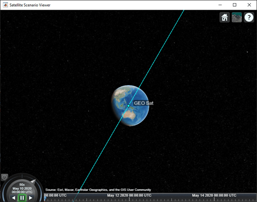
Add a ground track of the satellite to the visualization and adjust how much of the future and history of the ground track to display.
leadTime = 2*24*3600;                                          % seconds
trailTime = leadTime;
gt = groundTrack(sat,"LeadTime",leadTime,"TrailTime",trailTime)
gt =
  GroundTrack with properties:

          LeadTime: 172800
         TrailTime: 172800
         LineWidth: 1
     LeadLineColor: [1 1 0.0670]
    TrailLineColor: [1 1 0.0670]
    VisibilityMode: 'inherit'
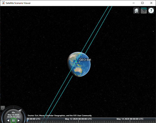
Visualize the satellite movement and its trace on the ground. The satellite covers the area around Japan during one half of the day and Australia during the other half.
play(sc);
Input Arguments
Name-Value Arguments
Specify optional pairs of arguments as
Name1=Value1,...,NameN=ValueN, where Name is
the argument name and Value is the corresponding value.
Name-value arguments must appear after other arguments, but the order of the
pairs does not matter.
Example: LeadTime=3600 sets the lead time of the ground track to 3600
seconds upon creation.
Satellite scenario viewer, specified as a scalar, vector, or array of satelliteScenarioViewer objects. If the AutoSimulate property of the scenario is false,
adding a satellite to the scenario disables any previously available timeline and
playback widgets.
Period of the ground track to be visualized in the Satellite Scenario Viewer, specified as a nonnegative scalar, in seconds.
The default value is for platforms and satellites whose
OrbitPropagator is set to 'ephemeris':
Satellite scenario
StartTimetoStopTimefor platforms and satellites whoseOrbitPropagatoris set to'ephemeris'For satellites in a parabolic or hyperbolic orbit and whose
OrbitPropagatoris set to'two-body-keplerian'or'numerical', the defaultLeadTimeis the duration from the satellite scenarioStartTimeto the time when the satellite reaches 145 times the equatorial radius of the central body.One orbital period, in all other cases.
In any case, ground tracks are not drawn on the Moon.
For splatforms with CentralBody set to "Moon",
ground track visualization is not supported. The TrailTime property is
accepted but has no visual effect.
Period of the ground track history to be visualized in the Satellite Scenario Viewer, specified as a positive scalar, in seconds.
The default value for platforms and satellites whose
OrbitPropagator is set to 'ephemeris':
Satellite scenario
StartTimetoStopTimewhenOrbitPropagatoris set to'ephemeris'For satellites in a parabolic or hyperbolic orbit and whose
OrbitPropagatoris set to'two-body-keplerian'or'numerical', the default TrailTime is the duration from the satellite scenario StartTime to the time when the satellite reaches 145 times the equatorial radius of the central body.One orbital period, in all other cases.
In any case, ground tracks are not drawn on the Moon.
For satellites or platforms with CentralBody set to
"Moon", ground track visualization is not supported in R2026b. The
TrailTime property is accepted but has no visual effect.
Visual width of the ground track in pixels, specified as 'LineWidth' and
a scalar in the range (0 10].
The line width cannot be thinner than the width of a pixel. If you set the line width to a value that is less than the width of a pixel on your system, the line displays as one pixel wide.
Color of the future ground track line, specified as 'LeadLineColor' and
an RGB triplet, a hexadecimal color code, a color name, or a short name.
For a custom color, specify an RGB triplet or a hexadecimal color code.
An RGB triplet is a three-element row vector whose elements specify the intensities of the red, green, and blue components of the color. The intensities must be in the range
[0,1], for example,[0.4 0.6 0.7].A hexadecimal color code is a string scalar or character vector that starts with a hash symbol (
#) followed by three or six hexadecimal digits, which can range from0toF. The values are not case sensitive. Therefore, the color codes"#FF8800","#ff8800","#F80", and"#f80"are equivalent.
Alternatively, you can specify some common colors by name. This table lists the named color options, the equivalent RGB triplets, and the hexadecimal color codes.
| Color Name | Short Name | RGB Triplet | Hexadecimal Color Code | Appearance |
|---|---|---|---|---|
"red"
|
"r"
|
[1 0 0]
|
"#FF0000"
|
|
"green"
|
"g"
|
[0 1 0]
|
"#00FF00"
|
|
"blue"
|
"b"
|
[0 0 1]
|
"#0000FF"
|
|
"cyan"
|
"c"
|
[0 1 1]
|
"#00FFFF"
|
|
"magenta"
|
"m"
|
[1 0 1]
|
"#FF00FF"
|
|
"yellow"
|
"y"
|
[1 1 0]
|
"#FFFF00"
|
|
"black"
|
"k"
|
[0 0 0]
|
"#000000"
|
|
"white"
|
"w"
|
[1 1 1]
|
"#FFFFFF"
|
|


Here are the RGB triplets and hexadecimal color codes for the default colors MATLAB® uses in many types of plots.
| RGB Triplet | Hexadecimal Color Code | Appearance |
|---|---|---|
[0 0.4470 0.7410]
|
"#0072BD"
|
|
[0.8500 0.3250 0.0980]
|
"#D95319"
|
|
[0.9290 0.6940 0.1250]
|
"#EDB120"
|
|
[0.4940 0.1840 0.5560]
|
"#7E2F8E"
|
|
[0.4660 0.6740 0.1880]
|
"#77AC30"
|
|
[0.3010 0.7450 0.9330]
|
"#4DBEEE"
|
|
[0.6350 0.0780 0.1840]
|
"#A2142F"
|
|
![Sample of RGB triplet [0 0.4470 0.7410], which appears as dark blue](colororder1.png)
![Sample of RGB triplet [0.8500 0.3250 0.0980], which appears as dark orange](colororder2.png)
![Sample of RGB triplet [0.9290 0.6940 0.1250], which appears as dark yellow](colororder3.png)
![Sample of RGB triplet [0.4940 0.1840 0.5560], which appears as dark purple](colororder4.png)
![Sample of RGB triplet [0.4660 0.6740 0.1880], which appears as medium green](colororder5.png)
![Sample of RGB triplet [0.3010 0.7450 0.9330], which appears as light blue](colororder6.png)
![Sample of RGB triplet [0.6350 0.0780 0.1840], which appears as dark red](colororder7.png)
Example: 'blue'
Example: [0 0 1]
Example: '#0000FF'
Color of the ground track line history, specified as 'TrailLineColor' and
an RGB triplet, a hexadecimal color code, a color name, or a short name.
For a custom color, specify an RGB triplet or a hexadecimal color code.
An RGB triplet is a three-element row vector whose elements specify the intensities of the red, green, and blue components of the color. The intensities must be in the range
[0,1], for example,[0.4 0.6 0.7].A hexadecimal color code is a string scalar or character vector that starts with a hash symbol (
#) followed by three or six hexadecimal digits, which can range from0toF. The values are not case sensitive. Therefore, the color codes"#FF8800","#ff8800","#F80", and"#f80"are equivalent.
Alternatively, you can specify some common colors by name. This table lists the named color options, the equivalent RGB triplets, and the hexadecimal color codes.
| Color Name | Short Name | RGB Triplet | Hexadecimal Color Code | Appearance |
|---|---|---|---|---|
"red"
|
"r"
|
[1 0 0]
|
"#FF0000"
|
|
"green"
|
"g"
|
[0 1 0]
|
"#00FF00"
|
|
"blue"
|
"b"
|
[0 0 1]
|
"#0000FF"
|
|
"cyan"
|
"c"
|
[0 1 1]
|
"#00FFFF"
|
|
"magenta"
|
"m"
|
[1 0 1]
|
"#FF00FF"
|
|
"yellow"
|
"y"
|
[1 1 0]
|
"#FFFF00"
|
|
"black"
|
"k"
|
[0 0 0]
|
"#000000"
|
|
"white"
|
"w"
|
[1 1 1]
|
"#FFFFFF"
|
|
Here are the RGB triplets and hexadecimal color codes for the default colors MATLAB uses in many types of plots.
| RGB Triplet | Hexadecimal Color Code | Appearance |
|---|---|---|
[0 0.4470 0.7410]
|
"#0072BD"
|
|
[0.8500 0.3250 0.0980]
|
"#D95319"
|
|
[0.9290 0.6940 0.1250]
|
"#EDB120"
|
|
[0.4940 0.1840 0.5560]
|
"#7E2F8E"
|
|
[0.4660 0.6740 0.1880]
|
"#77AC30"
|
|
[0.3010 0.7450 0.9330]
|
"#4DBEEE"
|
|
[0.6350 0.0780 0.1840]
|
"#A2142F"
|
|
Example: 'blue'
Example: [0 0 1]
Example: '#0000FF'
Default Values
The default value is:
[1 1 0.067]for satellite and platform[0.7483 0.7483 0.7483]for Moon
Limitations
Ground tracks are not drawn on the Moon surface in R2026b. Moon surface ground track rendering is not supported until a future release.

