fit

Train linear model for incremental learning

Since R2020b

Syntax

Mdl = fit(Mdl,X,Y)

Mdl = fit(Mdl,X,Y,Name,Value)

Description

The fit function fits a configured incremental learning model for linear regression (incrementalRegressionLinear object) or linear binary classification (incrementalClassificationLinear object) to streaming data. To additionally track performance metrics using the data as it arrives, use updateMetricsAndFit instead.

To fit or cross-validate a regression or classification model to an entire batch of data at once, see the other machine learning models in Regression or Classification.

Mdl = fit(Mdl,X,Y) returns an incremental learning model Mdl, which represents the input incremental learning model Mdl trained using the predictor and response data, X and Y respectively. Specifically, fit implements the following procedure:

1. Initialize the solver with the configurations and linear model coefficient and bias estimates of the input incremental learning model Mdl.

2. Fit the model to the data, and store the updated coefficient estimates and configurations in the output model Mdl.

The input and output models have the same data type.

Mdl = fit(Mdl,X,Y,Name,Value) uses additional options specified by one or more name-value pair arguments. For example, you can specify that the columns of the predictor data matrix correspond to observations, and set observation weights.

Examples

Incrementally Train Model

Create a default incremental linear SVM model for binary classification. Specify an estimation period of 5000 observations and the SGD solver.

Mdl = incrementalClassificationLinear('EstimationPeriod',5000,'Solver','sgd')

Mdl = 
  incrementalClassificationLinear

            IsWarm: 0
           Metrics: [1x2 table]
        ClassNames: [1x0 double]
    ScoreTransform: 'none'
              Beta: [0x1 double]
              Bias: 0
           Learner: 'svm'

Mdl is an incrementalClassificationLinear model. All its properties are read-only.

Mdl must be fit to data before you can use it to perform any other operations.

Load the human activity data set. Randomly shuffle the data.

load humanactivity
n = numel(actid);
rng(1) % For reproducibility
idx = randsample(n,n);
X = feat(idx,:);
Y = actid(idx);

For details on the data set, enter Description at the command line.

Responses can be one of five classes: Sitting, Standing, Walking, Running, or Dancing. Dichotomize the response by identifying whether the subject is moving (actid > 2).

Y = Y > 2;

Fit the incremental model to the training data, in chunks of 50 observations at a time, by using the fit function. At each iteration:

• Simulate a data stream by processing 50 observations.

• Overwrite the previous incremental model with a new one fitted to the incoming observations.

• Store ${\beta }_1$, the number of training observations, and the prior probability of whether the subject moved (Y = true) to see how they evolve during incremental training.

% Preallocation
numObsPerChunk = 50;
nchunk = floor(n/numObsPerChunk);
beta1 = zeros(nchunk,1);    
numtrainobs = zeros(nchunk,1);
priormoved = zeros(nchunk,1);

% Incremental fitting
for j = 1:nchunk
    ibegin = min(n,numObsPerChunk*(j-1) + 1);
    iend   = min(n,numObsPerChunk*j);
    idx = ibegin:iend;    
    Mdl = fit(Mdl,X(idx,:),Y(idx));
    beta1(j) = Mdl.Beta(1);
    numtrainobs(j) = Mdl.NumTrainingObservations; 
    priormoved(j) = Mdl.Prior(Mdl.ClassNames == true);
end

Mdl is an incrementalClassificationLinear model object trained on all the data in the stream.

To see how the parameters evolve during incremental learning, plot them on separate tiles.

tiledlayout(2,2)
nexttile
plot(beta1)
ylabel('\beta_1')
xline(Mdl.EstimationPeriod/numObsPerChunk,'r-.')
xlabel('Iteration')
axis tight
nexttile
plot(numtrainobs)
ylabel('Number of Training Observations')
xline(Mdl.EstimationPeriod/numObsPerChunk,'r-.')
xlabel('Iteration')
axis tight
nexttile
plot(priormoved)
ylabel('\pi(Subject Is Moving)')
xline(Mdl.EstimationPeriod/numObsPerChunk,'r-.')
xlabel('Iteration')
axis tight

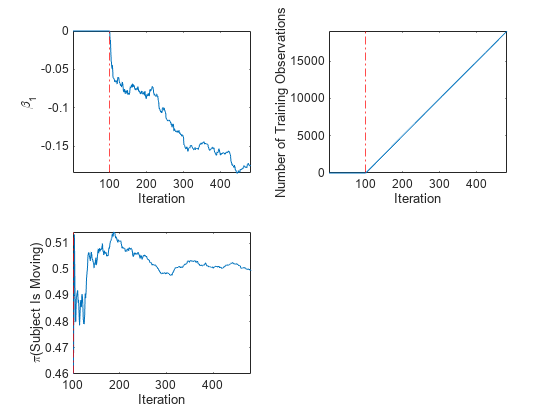
The plot suggests that fit does not fit the model to the data or update the parameters until after the estimation period.

Specify Orientation of Observations and Observation Weights

Train a linear model for binary classification by using fitclinear, convert it to an incremental learner, track its performance, and fit it to streaming data. Orient the observations in columns, and specify observation weights.

Load and Preprocess Data

Load the human activity data set. Randomly shuffle the data. Orient the observations of the predictor data in columns.

load humanactivity
rng(1); % For reproducibility
n = numel(actid);
idx = randsample(n,n);
X = feat(idx,:)';
Y = actid(idx);

For details on the data set, enter Description at the command line.

Responses can be one of five classes: Sitting, Standing, Walking, Running, or Dancing. Dichotomize the response by identifying whether the subject is moving (actid > 2).

Y = Y > 2;

Suppose that the data collected when the subject was not moving (Y = false) has double the quality than when the subject was moving. Create a weight variable that attributes 2 to observations collected from a still subject, and 1 to a moving subject.

W = ones(n,1) + ~Y;

Train Linear Model for Binary Classification

Fit a linear model for binary classification to a random sample of half the data.

idxtt = randsample([true false],n,true);
TTMdl = fitclinear(X(:,idxtt),Y(idxtt),'ObservationsIn','columns', ...
    'Weights',W(idxtt))

TTMdl = 
  ClassificationLinear
      ResponseName: 'Y'
        ClassNames: [0 1]
    ScoreTransform: 'none'
              Beta: [60x1 double]
              Bias: -0.1107
            Lambda: 8.2967e-05
           Learner: 'svm'

TTMdl is a ClassificationLinear model object representing a traditionally trained linear model for binary classification.

Convert Trained Model

Convert the traditionally trained classification model to a binary classification linear model for incremental learning.

IncrementalMdl = incrementalLearner(TTMdl)

IncrementalMdl = 
  incrementalClassificationLinear

            IsWarm: 1
           Metrics: [1x2 table]
        ClassNames: [0 1]
    ScoreTransform: 'none'
              Beta: [60x1 double]
              Bias: -0.1107
           Learner: 'svm'

Separately Track Performance Metrics and Fit Model

Perform incremental learning on the rest of the data by using the updateMetrics and fit functions. At each iteration:

1. Simulate a data stream by processing 50 observations at a time.

2. Call updateMetrics to update the cumulative and window classification error of the model given the incoming chunk of observations. Overwrite the previous incremental model to update the losses in the Metrics property. Note that the function does not fit the model to the chunk of data—the chunk is "new" data for the model. Specify that the observations are oriented in columns, and specify the observation weights.

3. Call fit to fit the model to the incoming chunk of observations. Overwrite the previous incremental model to update the model parameters. Specify that the observations are oriented in columns, and specify the observation weights.

4. Store the classification error and first estimated coefficient ${\beta }_1$.

% Preallocation
idxil = ~idxtt;
nil = sum(idxil);
numObsPerChunk = 50;
nchunk = floor(nil/numObsPerChunk);
ce = array2table(zeros(nchunk,2),'VariableNames',["Cumulative" "Window"]);
beta1 = [IncrementalMdl.Beta(1); zeros(nchunk,1)];
Xil = X(:,idxil);
Yil = Y(idxil);
Wil = W(idxil);

% Incremental fitting
for j = 1:nchunk
    ibegin = min(nil,numObsPerChunk*(j-1) + 1);
    iend   = min(nil,numObsPerChunk*j);
    idx = ibegin:iend;
    IncrementalMdl = updateMetrics(IncrementalMdl,Xil(:,idx),Yil(idx), ...
        'ObservationsIn','columns','Weights',Wil(idx));
    ce{j,:} = IncrementalMdl.Metrics{"ClassificationError",:};
    IncrementalMdl = fit(IncrementalMdl,Xil(:,idx),Yil(idx),'ObservationsIn','columns', ...
        'Weights',Wil(idx));
    beta1(j + 1) = IncrementalMdl.Beta(1);
end

IncrementalMdl is an incrementalClassificationLinear model object trained on all the data in the stream.

Alternatively, you can use updateMetricsAndFit to update performance metrics of the model given a new chunk of data, and then fit the model to the data.

Plot a trace plot of the performance metrics and estimated coefficient ${\beta }_1$.

t = tiledlayout(2,1);
nexttile
h = plot(ce.Variables);
xlim([0 nchunk])
ylabel('Classification Error')
legend(h,ce.Properties.VariableNames)
nexttile
plot(beta1)
ylabel('\beta_1')
xlim([0 nchunk])
xlabel(t,'Iteration')

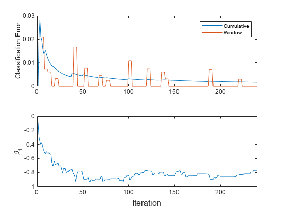
The cumulative loss is stable and gradually decreases, whereas the window loss jumps.

${\beta }_1$ changes gradually, then levels off, as fit processes more chunks.

Perform Conditional Training

Incrementally train a linear regression model only when its performance degrades.

Load and shuffle the 2015 NYC housing data set. For more details on the data, see NYC Open Data.

load NYCHousing2015

rng(1) % For reproducibility
n = size(NYCHousing2015,1);
shuffidx = randsample(n,n);
NYCHousing2015 = NYCHousing2015(shuffidx,:);

Extract the response variable SALEPRICE from the table. For numerical stability, scale SALEPRICE by 1e6.

Y = NYCHousing2015.SALEPRICE/1e6;
NYCHousing2015.SALEPRICE = [];

Create dummy variable matrices from the categorical predictors.

catvars = ["BOROUGH" "BUILDINGCLASSCATEGORY" "NEIGHBORHOOD"];
dumvarstbl = varfun(@(x)dummyvar(categorical(x)),NYCHousing2015, ...
    'InputVariables',catvars);
dumvarmat = table2array(dumvarstbl);
NYCHousing2015(:,catvars) = [];

Treat all other numeric variables in the table as linear predictors of sales price. Concatenate the matrix of dummy variables to the rest of the predictor data.

idxnum = varfun(@isnumeric,NYCHousing2015,'OutputFormat','uniform');
X = [dumvarmat NYCHousing2015{:,idxnum}];

Configure a linear regression model for incremental learning so that it does not have an estimation or metrics warm-up period. Specify a metrics window size of 1000. Fit the configured model to the first 100 observations.

Mdl = incrementalRegressionLinear('EstimationPeriod',0, ...
    'MetricsWarmupPeriod',0,'MetricsWindowSize',1000);
numObsPerChunk = 100;
Mdl = fit(Mdl,X(1:numObsPerChunk,:),Y(1:numObsPerChunk));

Mdl is an incrementalRegressionLinear model object.

Perform incremental learning, with conditional fitting, by following this procedure for each iteration:

• Simulate a data stream by processing a chunk of 100 observations at a time.

• Update the model performance by computing the epsilon insensitive loss, within a 200 observation window.

• Fit the model to the chunk of data only when the loss more than doubles from the minimum loss experienced.

• When tracking performance and fitting, overwrite the previous incremental model.

• Store the epsilon insensitive loss and ${\beta }_{313}$ to see how the loss and coefficient evolve during training.

• Track when fit trains the model.

% Preallocation
n = numel(Y) - numObsPerChunk;
nchunk = floor(n/numObsPerChunk);
beta313 = zeros(nchunk,1);
ei = array2table(nan(nchunk,2),'VariableNames',["Cumulative" "Window"]);
trained = false(nchunk,1);

% Incremental fitting
for j = 2:nchunk
    ibegin = min(n,numObsPerChunk*(j-1) + 1);
    iend   = min(n,numObsPerChunk*j);
    idx = ibegin:iend;
    Mdl = updateMetrics(Mdl,X(idx,:),Y(idx));
    ei{j,:} = Mdl.Metrics{"EpsilonInsensitiveLoss",:};
    minei = min(ei{:,2});
    pdiffloss = (ei{j,2} - minei)/minei*100;
    if pdiffloss > 100
        Mdl = fit(Mdl,X(idx,:),Y(idx));
        trained(j) = true;
    end    
    beta313(j) = Mdl.Beta(end);
end

Mdl is an incrementalRegressionLinear model object trained on all the data in the stream.

To see how the model performance and ${\beta }_{313}$ evolve during training, plot them on separate tiles.

t = tiledlayout(2,1);
nexttile
plot(beta313)
hold on
plot(find(trained),beta313(trained),'r.')
xlim([0 nchunk])
ylabel('\beta_{313}')
xline(Mdl.EstimationPeriod/numObsPerChunk,'r-.')
legend('\beta_{313}','Training occurs','Location','southeast')
hold off
nexttile
plot(ei.Variables)
xlim([0 nchunk])
ylabel('Epsilon Insensitive Loss')
xline(Mdl.EstimationPeriod/numObsPerChunk,'r-.')
legend(ei.Properties.VariableNames)
xlabel(t,'Iteration')

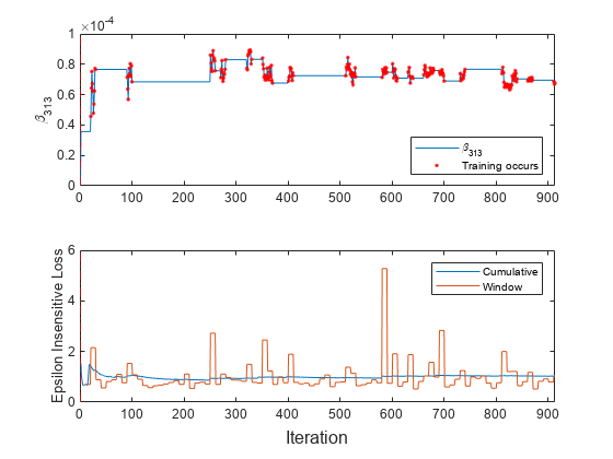
The trace plot of ${\beta }_{313}$ shows periods of constant values, during which the loss did not double from the minimum experienced.

Input Arguments

Mdl — Incremental learning model

incrementalClassificationLinear model object | incrementalRegressionLinear model object

Incremental learning model to fit to streaming data, specified as an incrementalClassificationLinear or incrementalRegressionLinear model object. You can create Mdl directly or by converting a supported, traditionally trained machine learning model using the incrementalLearner function. For more details, see the corresponding reference page.

X — Chunk of predictor data

floating-point matrix

Chunk of predictor data to which the model is fit, specified as a floating-point matrix of n observations and Mdl.NumPredictors predictor variables. The value of the ObservationsIn name-value argument determines the orientation of the variables and observations. The default ObservationsIn value is "rows", which indicates that observations in the predictor data are oriented along the rows of X.

The length of the observation labels Y and the number of observations in X must be equal; Y(j) is the label of observation j (row or column) in X.

Note

• If Mdl.NumPredictors = 0, fit infers the number of predictors from X, and sets the corresponding property of the output model. Otherwise, if the number of predictor variables in the streaming data changes from Mdl.NumPredictors, fit issues an error.

• fit supports only floating-point input predictor data. If your input data includes categorical data, you must prepare an encoded version of the categorical data. Use dummyvar to convert each categorical variable to a numeric matrix of dummy variables. Then, concatenate all dummy variable matrices and any other numeric predictors. For more details, see Dummy Variables.

Data Types: single | double

Y — Chunk of responses (labels)

categorical array | character array | string array | logical vector | floating-point vector | cell array of character vectors

Chunk of responses (labels) to which the model is fit, specified as a categorical, character, or string array, logical or floating-point vector, or cell array of character vectors for classification problems; or a floating-point vector for regression problems.

The length of the observation labels Y and the number of observations in X must be equal; Y(j) is the label of observation j (row or column) in X.

For classification problems:

• fit supports binary classification only.

• When the ClassNames property of the input model Mdl is nonempty, the following conditions apply:

  • If Y contains a label that is not a member of Mdl.ClassNames, fit issues an error.

  • The data type of Y and Mdl.ClassNames must be the same.

Data Types: char | string | cell | categorical | logical | single | double

Note

• If an observation (predictor or label) or weight contains at least one missing (NaN) value, fit ignores the observation. Consequently, fit uses fewer than n observations to create an updated model, where n is the number of observations in X.

• The chunk size n and the stochastic gradient descent (SGD) hyperparameter mini-batch size (Mdl.BatchSize) can be different values, and n does not have to be an exact multiple of the mini-batch size. If n < Mdl.BatchSize, fit uses the n available observations when it applies SGD. If n > Mdl.BatchSize, the function updates the model with a mini-batch of the specified size multiple times, and then uses the rest of the observations for the last mini-batch. The number of observations for the last mini-batch can be smaller than Mdl.BatchSize.

Name-Value Arguments

Specify optional pairs of arguments as Name1=Value1,...,NameN=ValueN, where Name is the argument name and Value is the corresponding value. Name-value arguments must appear after other arguments, but the order of the pairs does not matter.

Before R2021a, use commas to separate each name and value, and enclose Name in quotes.

Example: 'ObservationsIn','columns','Weights',W specifies that the columns of the predictor matrix correspond to observations, and the vector W contains observation weights to apply during incremental learning.

ObservationsIn — Predictor data observation dimension

'rows' (default) | 'columns'

Predictor data observation dimension, specified as the comma-separated pair consisting of 'ObservationsIn' and 'columns' or 'rows'.

Data Types: char | string

Weights — Chunk of observation weights

floating-point vector of positive values

Chunk of observation weights, specified as the comma-separated pair consisting of 'Weights' and a floating-point vector of positive values. fit weighs the observations in X with the corresponding values in Weights. The size of Weights must equal n, which is the number of observations in X.

By default, Weights is ones(n,1).

For more details, including normalization schemes, see Observation Weights.

Data Types: double | single

Output Arguments

Mdl — Updated incremental learning model

incrementalClassificationLinear model object | incrementalRegressionLinear model object

Updated incremental learning model, returned as an incremental learning model object of the same data type as the input model Mdl, either incrementalClassificationLinear or incrementalRegressionLinear.

If Mdl.EstimationPeriod > 0, the incremental fitting functions updateMetricsAndFit and fit estimate hyperparameters using the first Mdl.EstimationPeriod observations passed to either function; they do not train the input model to that data. However, if an incoming chunk of n observations is greater than or equal to the number of observations remaining in the estimation period m, fit estimates hyperparameters using the first n – m observations, and fits the input model to the remaining m observations. Consequently, the software updates the Beta and Bias properties, hyperparameter properties, and recordkeeping properties such as NumTrainingObservations.

For classification problems, if the ClassNames property of the input model Mdl is an empty array, fit sets the ClassNames property of the output model Mdl to unique(Y).

Tips

• Unlike traditional training, incremental learning might not have a separate test (holdout) set. Therefore, to treat each incoming chunk of data as a test set, pass the incremental model and each incoming chunk to updateMetrics before training the model on the same data.

Algorithms

Observation Weights

For classification problems, if the prior class probability distribution is known (in other words, the prior distribution is not empirical), fit normalizes observation weights to sum to the prior class probabilities in the respective classes. This action implies that observation weights are the respective prior class probabilities by default.

For regression problems or if the prior class probability distribution is empirical, the software normalizes the specified observation weights to sum to 1 each time you call fit.

Extended Capabilities

C/C++ Code Generation

Generate C and C++ code using MATLAB® Coder™.

Usage notes and limitations:

• Use saveLearnerForCoder, loadLearnerForCoder, and codegen (MATLAB Coder) to generate code for the fit function. Save a trained model by using saveLearnerForCoder. Define an entry-point function that loads the saved model by using loadLearnerForCoder and calls the fit function. Then use codegen to generate code for the entry-point function.

• To generate single-precision C/C++ code for fit, specify the name-value argument "DataType","single" when you call the loadLearnerForCoder function.

• This table contains notes about the arguments of fit. Arguments not included in this table are fully supported.

  Argument	Notes and Limitations
  Mdl	For usage notes and limitations of the model object, see incrementalClassificationLinear or incrementalRegressionLinear.
  X	Batch-to-batch, the number of observations can be a variable size, but must equal the number of observations in Y. The number of predictor variables must equal to Mdl.NumPredictors. X must be single or double.
  Y	Batch-to-batch, the number of observations can be a variable size, but must equal the number of observations in X. For classification problems, all labels in Y must be represented in Mdl.ClassNames. Y and Mdl.ClassNames must have the same data type.

• The following restrictions apply:

  • If you configure Mdl to shuffle data (Mdl.Shuffle is true, or Mdl.Solver is 'sgd' or 'asgd'), the fit function randomly shuffles each incoming batch of observations before it fits the model to the batch. The order of the shuffled observations might not match the order generated by MATLAB^®. Therefore, the fitted coefficients computed in MATLAB and the generated code might not be equal.

  • Use a homogeneous data type for all floating-point input arguments and object properties, specifically, either single or double.

For more information, see Introduction to Code Generation.

Version History

Introduced in R2020b