cos

Symbolic cosine function

collapse all in page

Syntax

cos(X)

Description

cos(X) returns the cosine function of X.

example

Examples

Cosine Function for Numeric and Symbolic Arguments

Depending on its arguments, cos returns floating-point or exact symbolic results.

Compute the cosine function for these numbers. Because these numbers are not symbolic objects, cos returns floating-point results.

A = cos([-2, -pi, pi/6, 5*pi/7, 11])

A =
   -0.4161   -1.0000    0.8660   -0.6235    0.0044

Compute the cosine function for the numbers converted to symbolic objects. For many symbolic (exact) numbers, cos returns unresolved symbolic calls.

symA = cos(sym([-2, -pi, pi/6, 5*pi/7, 11]))

symA =
[ cos(2), -1, 3^(1/2)/2, -cos((2*pi)/7), cos(11)]

Use vpa to approximate symbolic results with floating-point numbers:

vpa(symA)

ans =
[ -0.41614683654714238699756822950076,...
-1.0,...
0.86602540378443864676372317075294,...
-0.62348980185873353052500488400424,...
0.0044256979880507857483550247239416]

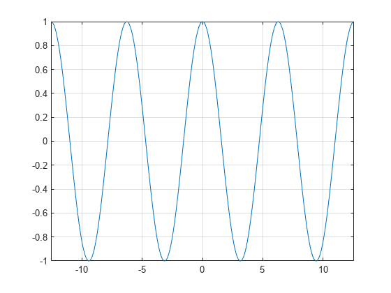
Plot Cosine Function

Plot the cosine function on the interval from $- 4 π$ to $4 π$ .

syms x
fplot(cos(x),[-4*pi 4*pi])
grid on

Figure contains an axes object. The axes object contains an object of type functionline.

Handle Expressions Containing Cosine Function

Many functions, such as diff, int, taylor, and rewrite, can handle expressions containing cos.

Find the first and second derivatives of the cosine function:

syms x
diff(cos(x), x)
diff(cos(x), x, x)

ans =
-sin(x)
 
ans =
-cos(x)

Find the indefinite integral of the cosine function:

int(cos(x), x)

ans =
sin(x)

Find the Taylor series expansion of cos(x):

taylor(cos(x), x)

ans =
x^4/24 - x^2/2 + 1

Rewrite the cosine function in terms of the exponential function:

rewrite(cos(x), 'exp')

ans =
exp(-x*1i)/2 + exp(x*1i)/2

Evaluate Units with `cos` Function

cos numerically evaluates these units automatically: radian, degree, arcmin, arcsec, and revolution.

Show this behavior by finding the cosine of x degrees and 2 radians.

u = symunit;
syms x
f = [x*u.degree 2*u.radian];
cosinf = cos(f)

cosinf =
[ cos((pi*x)/180), cos(2)]

You can calculate cosinf by substituting for x using subs and then using double or vpa.

Input Arguments

collapse all

`X` — Input
symbolic number | symbolic scalar variable | symbolic matrix variable | symbolic expression | symbolic function | symbolic matrix function | symbolic vector | symbolic matrix

Input, specified as a symbolic number, scalar variable, matrix variable, expression, function, matrix function, or as a vector or matrix of symbolic numbers, scalar variables, expressions, or functions.

More About

collapse all

Cosine Function

The cosine of an angle, α, defined with reference to a right triangle is

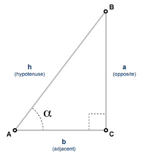
$cos (α) = \frac{adjacent side}{hypotenuse} = \frac{b}{h} .$

Right triangle with vertices A, B, and C. The vertex A has an angle α, and the vertex C has a right angle. The hypotenuse, or side AB, is labeled as h. The opposite side of α, or side BC, is labeled as a. The adjacent side of α, or side AC, is labeled as b. The cosine of α is defined as the adjacent side b divided by the hypotenuse h.

The cosine of a complex argument, α, is

$cos (α) = \frac{e^{i α} + e^{- i α}}{2} .$

Version History

Introduced before R2006a

expand all

R2022a: Compute cosine of symbolic matrix functions

The cos function accepts an input argument of type symfunmatrix.

R2021a: Compute cosine of symbolic matrix variables

The cos function accepts an input argument of type symmatrix.

cos