biorwavf
Biorthogonal spline wavelet filter
Description
Examples
Return the biorthogonal spline wavelet scaling filters with two vanishing moments.
wname = 'bior2.2';
[RF,DF] = biorwavf(wname)
RF = 1×3
0.2500 0.5000 0.2500
DF = 1×5

   -0.1250    0.2500    0.7500    0.2500   -0.1250
This example shows how to take analysis and synthesis filters associated with a biorthogonal wavelet and make them compatible with Wavelet Toolbox™. Wavelet Toolbox requires that analysis and synthesis lowpass and highpass filters have equal even length. This example uses the nearly orthogonal biorthogonal wavelets based on the Laplacian pyramid scheme of Burt and Adelson (Table 8.4 on page 283 in [1]). The example also demonstrates how to examine properties of the biorthogonal wavelets.
Define the analysis and synthesis filter coefficients of the biorthogonal wavelet.
Hd = [-1 5 12 5 -1]/20*sqrt(2);
Gd = [3 -15 -73 170 -73 -15 3]/280*sqrt(2);
Hr = [-3 -15 73 170 73 -15 -3]/280*sqrt(2);
Gr = [-1 -5 12 -5 -1]/20*sqrt(2);
Hd and Gd are the lowpass and highpass analysis filters, respectively. Hr and Gr are the lowpass and highpass synthesis filters. They are all finite impulse response (FIR) filters. Confirm the lowpass filter coefficients sum to sqrt(2) and the highpass filter coefficients sum to 0.
sum(Hd)/sqrt(2)
ans =
1.0000
sum(Hr)/sqrt(2)
ans =
1.0000
sum(Gd)
ans =
-1.0061e-16
sum(Gr)
ans =
-9.7145e-17
The z-transform of an FIR filter is a Laurent polynomial given by . The degree of a Laurent polynomial is defined as . Therefore, the length of the filter is . Examine the Laurent expansion of the scaling and wavelet filters.
PHd = laurentPolynomial(Coefficients=Hd,MaxOrder=2)
PHd =
  laurentPolynomial with properties:

    Coefficients: [-0.0707 0.3536 0.8485 0.3536 -0.0707]
        MaxOrder: 2
PHr = laurentPolynomial(Coefficients=Hr,MaxOrder=3)
PHr =
  laurentPolynomial with properties:

    Coefficients: [-0.0152 -0.0758 0.3687 0.8586 0.3687 -0.0758 -0.0152]
        MaxOrder: 3
PGd = laurentPolynomial(Coefficients=Gd,MaxOrder=3)
PGd =
  laurentPolynomial with properties:

    Coefficients: [0.0152 -0.0758 -0.3687 0.8586 -0.3687 -0.0758 0.0152]
        MaxOrder: 3
PGr = laurentPolynomial(Coefficients=Gr,MaxOrder=2)
PGr =
  laurentPolynomial with properties:

    Coefficients: [-0.0707 -0.3536 0.8485 -0.3536 -0.0707]
        MaxOrder: 2
Since the filters are associated with biorthogonal wavelet, confirm .
PHd*PHr + PGd*PGr
ans =
  laurentPolynomial with properties:

    Coefficients: 2
        MaxOrder: 0
Wavelet Toolbox™ requires that filters associated with the wavelet have even equal length. To use the Laplacian wavelet filters in the toolbox, you must include the missing powers of the Laurent series as zeros.
The degrees of PHd and PHr are 4 and 6, respectively. The minimum even-length filter that can accommodate the four filters has length 8, which corresponds to a Laurent polynomial of degree 7. The strategy is to prepend and append 0s as evenly as possible so that all filters are of length 8. Prepend 0 to all the filters, and then append two 0s to Hd and Gr.
Hd = [0 Hd 0 0];
Gd = [0 Gd];
Hr = [0 Hr];
Gr = [0 Gr 0 0];
You can examine properties of the biorthogonal wavelets by creating DWT filter banks. Create two custom DWT filter banks using the filters, one for analysis and the other for synthesis. Confirm the filter banks are biorthogonal.
fb = dwtfilterbank('Wavelet','Custom',...
    'CustomScalingFilter',[Hd' Hr'],...
    'CustomWaveletFilter',[Gd' Gr']);

fb2 = dwtfilterbank('Wavelet','Custom',...
    'CustomScalingFilter',[Hd' Hr'],...
    'CustomWaveletFilter',[Gd' Gr'],...
    'FilterType','Synthesis');

fprintf('fb: isOrthogonal = %d\tisBiorthogonal = %d\n',...
    isOrthogonal(fb),isBiorthogonal(fb));
fb: isOrthogonal = 0 isBiorthogonal = 1
fprintf('fb2: isOrthogonal = %d\tisBiorthogonal = %d\n',...
    isOrthogonal(fb2),isBiorthogonal(fb2));
fb2: isOrthogonal = 0 isBiorthogonal = 1
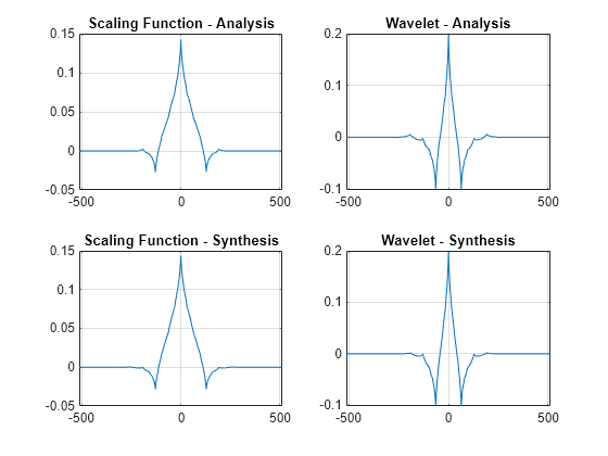
Plot the scaling and wavelet functions associated with the filter banks at the coarsest scale.
[phi,t] = scalingfunctions(fb);
[psi,~] = wavelets(fb);
[phi2,~] = scalingfunctions(fb2);
[psi2,~] = wavelets(fb2);
subplot(2,2,1)
plot(t,phi(end,:))
grid on
title('Scaling Function - Analysis')
subplot(2,2,2)
plot(t,psi(end,:))
grid on
title('Wavelet - Analysis')
subplot(2,2,3)
plot(t,phi2(end,:))
grid on
title('Scaling Function - Synthesis')
subplot(2,2,4)
plot(t,psi2(end,:))
grid on
title('Wavelet - Synthesis')

Compute the filter bank framebounds.
[analysisLowerBound,analysisUpperBound] = framebounds(fb)
analysisLowerBound =
0.9505
analysisUpperBound =
1.0211
[synthesisLowerBound,synthesisUpperBound] = framebounds(fb2)
synthesisLowerBound =
0.9800
synthesisUpperBound =
1.0528
Input Arguments
Name of biorthogonal wavelet, specified as 'biorNr.Nd'
where possible values for Nr and Nd
are as follows:
Nr = 1 | Nd = 1 , 3 or 5 |
Nr = 2 | Nd = 2 , 4 , 6 or 8 |
Nr = 3 | Nd = 1 , 3 , 5 , 7 or 9 |
Nr = 4 | Nd = 4 |
Nr = 5 | Nd = 5 |
Nr = 6 | Nd = 8 |
Nr and Nd are the
numbers of vanishing moments for the reconstruction and decomposition
filters, respectively.
Example: 'biorwavf3.7'
Output Arguments
Version History
Introduced before R2006a
MATLAB Command
You clicked a link that corresponds to this MATLAB command:
Run the command by entering it in the MATLAB Command Window. Web browsers do not support MATLAB commands.
Seleccione un país/idioma
Seleccione un país/idioma para obtener contenido traducido, si está disponible, y ver eventos y ofertas de productos y servicios locales. Según su ubicación geográfica, recomendamos que seleccione: .
También puede seleccionar uno de estos países/idiomas:
Cómo obtener el mejor rendimiento
Seleccione China (en idioma chino o inglés) para obtener el mejor rendimiento. Los sitios web de otros países no están optimizados para ser accedidos desde su ubicación geográfica.
América
- América Latina (Español)
- Canada (English)
- United States (English)
Europa
- Belgium (English)
- Denmark (English)
- Deutschland (Deutsch)
- España (Español)
- Finland (English)
- France (Français)
- Ireland (English)
- Italia (Italiano)
- Luxembourg (English)
- Netherlands (English)
- Norway (English)
- Österreich (Deutsch)
- Portugal (English)
- Sweden (English)
- Switzerland
- United Kingdom (English)