Optimize Wi-Fi Networks Using MATLAB

Since R2026a

This example shows how to optimize the layout of an IEEE® 802.11 (Wi-Fi®) [1] network to satisfy throughput requirements.

Using this example, you can:

1. Formulate an optimization problem to adjust the number and placement of access points (APs) to achieve a given minimum throughput for each station (STA).

2. Create a Wi-Fi network with a fixed number of STAs and APs across a defined area.

3. Solve the optimization problem using the surrogate optimization solver.

The results identify the optimal number and placement of APs to meet the throughput requirements for each STA.

Additionally, you can also use this example script to explore different optimization options.

Wi-Fi Network Layout

The example optimizes AP placement to ensure that each of the four STAs achieve at least 20 Mbps throughput. It simulates the network over a 40-by-40-meter area (160 square meters). Additionally, the example shows results from a scenario with 16 STAs and up to six available APs.

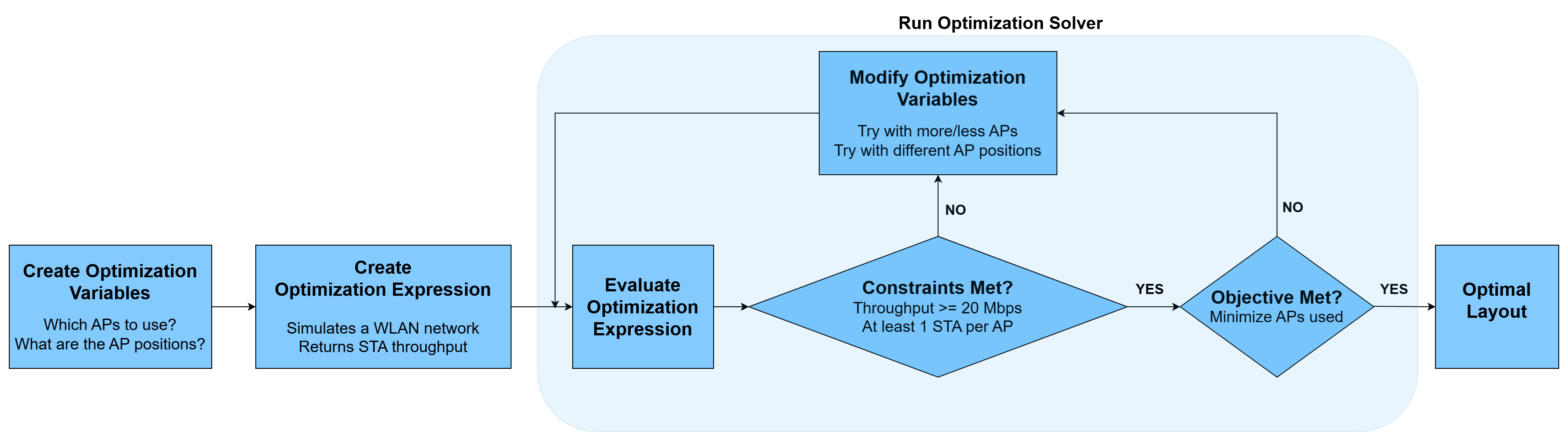
This optimization process consists of these steps:

1. Create optimization variables — Create variables defining which APs to use out of all available APs, and where to place them.

2. Create optimization expression — Create a function to simulate Wi-Fi network and return throughput at each STA.

3. Run optimization solver — Pick values for number of APs used and their positions, simulate the Wi-Fi network and check if throughput requirement is met at all STAs. Repeat the process several times, each time using different number of APs located at different positions to optimize the layout.

Simulation Configuration

Set the random number generator seed to 1 to produce a consistent layout across repeated runs of the example. This seed value determines the random number pattern, which in turn controls the STA placement and the resulting optimal AP positions.

rngSeed = 1;
rng(rngSeed,"combRecursive")

Specify the length (x-axis) and breadth (y-axis) of the available area, in meters.

scenarioLength = 40;
scenarioBreadth = 40;
scenarioArea = scenarioLength*scenarioBreadth;

Specify the number of APs available for use.

maxNumAPs = 2;

Specify the number of STAs that the APs serve in the scenario area.

numSTAs = 4;

Specify the simulation time of the Wi-Fi network, in seconds.

simulationTime = 0.5;

Optimization Process

Global Optimization Toolbox supports two optimization approaches: problem-based and solver-based. This example uses the problem-based approach because it is easier to set up and use, and it meets the requirements of this example. For more information on selecting an approach for your optimization problem, see Decide Between Problem-Based and Solver-Based Approach (Global Optimization Toolbox).

Create Optimization Variables

Identify the variables you must adjust to achieve an optimized layout. In this example, the number of active APs and their positions serve as the optimization variables. To create these variables, use the optimvar (Optimization Toolbox) object. Specify any bounds within the variable definitions. The solver adjusts these variables during each run to find an optimal value.

Specify the apEnable variable as a logical vector of size maxNumAPs-by-1, to indicate which available APs the simulation uses.

apEnable = optimvar("apEnable",maxNumAPs,1,LowerBound=0,UpperBound=1,Type="integer");

Specify the Cartesian x- and y-coordinates for all APs by creating vector variables, apXPosition and apYPosition, each of size maxNumAPs-by-1. Constrain these coordinates to the scenario area by setting their lower and upper bounds to match the dimensions of the scenario area. For ease of use, you can optionally restrict these coordinates to integer values.

apXPosition = optimvar("apXPosition",maxNumAPs,1,LowerBound=0,UpperBound=scenarioLength,Type="integer");
apYPosition = optimvar("apYPosition",maxNumAPs,1,LowerBound=0,UpperBound=scenarioBreadth,Type="integer");
apPositions = [apXPosition apYPosition 3*ones(maxNumAPs,1)]; % Z-coordinate is fixed

Create a fixed layout for the STAs by using the local getSTAPositions function to retrieve random Cartesian x-, y-, and z-coordinates for each STA. You can modify this function to generate a custom STA layout.

staPositions = getSTAPositions(numSTAs,scenarioLength,scenarioBreadth);

Create Optimization Expression

Create an optimization expression using the optimization variables. The solver evaluates this expression by testing different variable values to minimize the number of APs while satisfying the throughput requirement at each STA. This example uses the local function simulateWLANNetwork as the optimization expression. This function creates a Wi-Fi network, with a specified number of APs and STAs, and returns the throughput at each STA. In each simulation run, each STA always associates to its nearest AP. Each AP and STA operates on a 20 MHz channel, uses a fixed modulation and coding scheme (MCS) of 9, and uses a single spatial stream. Under these conditions, and in accordance with the IEEE 802.11ax™ specification [1], a node can deliver a maximum physical layer (PHY) data rate of 97.5 Mbps when it communicates with a single receiver. If an AP serves multiple STAs, it splits this data rate among them.

To convert the local function into an optimization expression, use the fcn2optimexpr (Optimization Toolbox) function. To avoid recalculating the objective and constraints, specify the ReuseEvaluation argument as true. To treat the function as a black box, specify the Analysis argument as "off".

[staThroughput,numSTAsPerAP] = fcn2optimexpr(@simulateWLANNetwork,apEnable,apPositions,staPositions,simulationTime,rngSeed,ReuseEvaluation=true,Analysis="off");

Create Optimization Problem

Create an optimization problem object, by using the optimproblem (Optimization Toolbox) function, to hold the objective expression and constraints. Specify the objective as minimizing the number of active APs.

problem = optimproblem(Objective=sum(apEnable),ObjectiveSense="minimize"); % sum(apEnable) gives the number of active APs

To specify a constraint, populate the Constraints structure of the optimization problem object. Create a field for each constraint and specify the expression that defines the constraint. The example defines three constraints, named: MustHaveOneAP, NumSTAsPerAP, and LowerLimitofSTAThroughput.

problem.Constraints.MustHaveOneAP = (sum(apEnable) >= 1);              % Enable at least one AP
problem.Constraints.NumSTAsPerAP = (numSTAsPerAP >= apEnable);         % Each enabled AP must serve at least one STA
problem.Constraints.LowerLimitofSTAThroughput = (staThroughput >= 20); % Minimum throughput at each STA must be 20 Mbps

Solve Optimization Problem

You can use the Surrogate Optimization (Global Optimization Toolbox) solver to seek the global minimum of an objective function while keeping the number of evaluations low. Surrogate optimization does this by approximating the objective function and sampling it at many points. Set the optimization options MaxFunctionEvaluations and MinSurrogatePoints by using the optimoptions (Optimization Toolbox) function. When you optimize a scenario with more STAs, you must increase the number of evaluations to help the solver reach an optimized solution. For example, in a scenario with eight STAs, you might increase MaxFunctionEvaluations value to 100. If you want to enable parallel evaluations by using the UseParallel option, you must have a Parallel Computing Toolbox™ license.

opts = optimoptions("surrogateopt", ...
    MaxFunctionEvaluations=10, ... % Maximum evaluations of the objective before stopping
    MinSurrogatePoints=24, ...     % Minimum number of initial sample points
    UseParallel=false);            % Parallel evaluations

Solve the optimization problem by using the solve (Optimization Toolbox) function. The sol output returns the final values for the optimization variables apEnable, apXPosition, and apYPosition. The fval output returns the final value of the objective, which is the number of active APs used in the simulation.

[sol,fval] = solve(problem,Solver="surrogateopt",Options=opts)

Solving problem using surrogateopt.

surrogateopt stopped because it exceeded the function evaluation limit set by 
'options.MaxFunctionEvaluations'.

sol = struct with fields:
       apEnable: [2×1 double]
    apXPosition: [2×1 double]
    apYPosition: [2×1 double]

fval = 
1

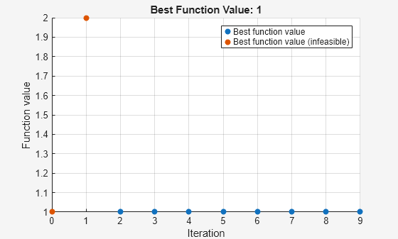
The solver displays its progress as a line plot showing the objective function value (number of APs) at each iteration of the simulation. In each iteration, the solver attempts to minimize the number of APs by running the simulation with different values for the optimization variables and checking whether the solution satisfies all constraints. Feasible solutions satisfy all constraints and appear as blue dots. A feasible value of 1 means the solver identified a single AP as sufficient to provide at least 20 Mbps throughput at each STA. The solver stops after 10 iterations because the MaxFunctionEvaluations value is 10. For more information about the surrogate optimization steps, see Interpret surrogateoptplot (Global Optimization Toolbox).

Simulation Results

Visualize the optimized layouts of these network scenarios.

• Two available APs and four STAs

• Six available APs and 16 STAs

Optimized Layout for Two Available APs and Four STAs

To view the optimized network layout, create a wirelessNetworkViewer object. Plot the positions of the AP and STAs by using the addNodes object function of the wirelessNetworkViewer object.

viewerObj = wirelessNetworkViewer;
solvedAPPositions = [sol.apXPosition sol.apYPosition 3*ones(maxNumAPs,1)];
enabledAPPositions = solvedAPPositions(logical(sol.apEnable),:);
addNodes(viewerObj,enabledAPPositions,Type="AP",Name="AP"+(1:size(enabledAPPositions,1)))
addNodes(viewerObj,staPositions,Type="STA",Name="STA"+(1:size(staPositions,1)))

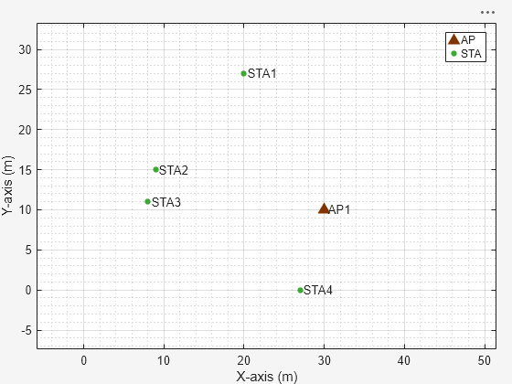
The solver determines the AP layout that best balances coverage and interference for the given STA locations. The above layout shows the most efficient AP deployment that meets the design requirement.

Calculate the throughput, in Mbps, for each STA to verify that each one meets the 20 Mbps throughput constraint when using the optimized AP placement.

[solvedSTAThroughput,~] = simulateWLANNetwork(sol.apEnable,solvedAPPositions,staPositions,simulationTime,rngSeed)

solvedSTAThroughput = 1×4

   22.7040   22.7040   21.6720   21.6720

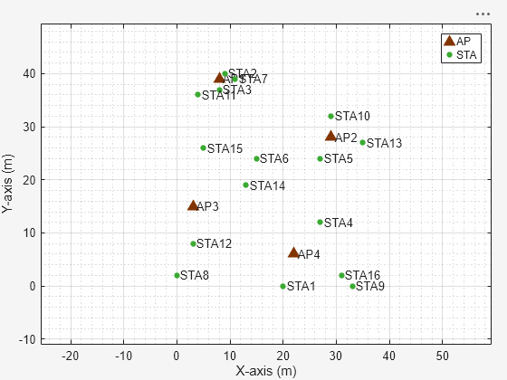
Optimized Layout for 6 Available APs and 16 STAs

This scenario increases the number of APs, which also increases the network complexity. The sizes of the optimization variables apXPosition and apYPosition each increase to 6-by-1. Therefore, you must adjust the example configuration to help the solver find an optimized solution.

To obtain the optimized layout, run the example again with these parameters.

• simulationTime — Set this value to 1 second. Running the simulation for a longer duration provides more accurate results.

• MaxFunctionEvaluations — Set this value to 200. Increasing this value enables the solver to evaluate the objective function more times.

• MinSurrogatePoints — Set this value to 40. Increasing this value helps the solver build a more accurate surrogate model.

If you run the example with these parameters, the solver uses four APs to satisfy all constraints. The example stores the results in the StoredResults16STAs.mat file. To view the optimal layout for this configuration, use a wirelessNetworkViewer object to plot the AP and STA positions retrieved from the MAT file.

load("StoredResults16STAs.mat")
newViewerObj = wirelessNetworkViewer;
addNodes(newViewerObj,storedAPPositions,Type="AP",Name="AP"+(1:size(storedAPPositions,1)))
addNodes(newViewerObj,storedSTAPositions,Type="STA",Name="STA"+(1:size(storedSTAPositions,1)))

Calculate the throughput, in Mbps, for each STA to verify that each STA meets the throughput constraint of 20 Mbps upon using the optimized placement of the APs.

storedThroughputs

storedThroughputs = 1×16

   22.7040   22.7040   22.1880   22.1880   22.7040   22.1880   22.1880   22.7040   22.1880   22.1880   22.1880   22.1880   22.1880   22.1880   22.1880   22.1880

Further Exploration

You can use this example to further explore these capabilities.

Adjust Optimization Options

The surrogate optimization solver provides various optimization options, which can be adjusted to better suit your design problem.

• MaxFunctionEvaluations — Use this criterion to stop the solver after it evaluates the objective function a specified number of times. This option helps you control run time in long simulations.

• MinSurrogatePoints — The surrogate algorithm initializes a set of random sample points for the optimization variables, evaluates the objective function at these points, and uses the results to construct a surrogate model. By default, the solver sets MinSurrogatePoints to max(20,2*nvar), where nvar is the number of optimization problem variables. Increasing this value usually helps the solver build a more accurate surrogate, but increases the number of objective function evaluations. For more information, see Surrogate Optimization Algorithm (Global Optimization Toolbox).

• ObjectiveLimit — Use this tolerance on the objective function value to stop the algorithm when it finds a feasible point where the objective function value falls below ObjectiveLimit. This option is useful when you know a typical "best" value of the objective function that satisfies your design goals.

Appendix

This example uses these helper objects included as supporting files, to create a wireless channel model for the Wi-Fi network.

• hSLSTGaxMultiFrequencySystemChannel — Creates a system channel object

• hSLSTGaxAbstractSystemChannel — Creates a channel object for an abstracted PHY layer

• hSLSTGaxSystemChannel — Creates a channel object for a full PHY layer

• hSLSTGaxSystemChannelBase — Creates the base channel object

References

1. “IEEE Standard for Information Technology–Telecommunications and Information Exchange between Systems Local and Metropolitan Area Networks–Specific Requirements Part 11: Wireless LAN Medium Access Control (MAC) and Physical Layer (PHY) Specifications.” IEEE Std 802.11-2024 (Revision of IEEE Std 802.11-2020), April 2025, 1–5956. https://doi.org/10.1109/IEEESTD.2025.10979691.

Local Functions

simulateWLANNetwork

Create, configure, and simulate a Wi-Fi network by using the simulateWLANNetwork function. This function uses the System-Level Simulation capabilities of WLAN Toolbox™. For more information, see the Get Started with WLAN System-Level Simulation in MATLAB example. The network configuration includes these specifications.

• Each AP operates on a dedicated 20 MHz channel in the 5 GHz band, and each STA uses the same channel as its closest associated AP.

• Each WLAN node uses a fixed MCS of 9, a single spatial stream, and a transmission power of 10 dBm.

• Each AP generates continuous downlink full-buffer application traffic.

The example models a random TGax fading channel between nodes using the hSLSTGaxMultiFrequencySystemChannel helper object.

function [stationThroughput,numSTAsPerAP] = simulateWLANNetwork(enableAP,apPositions,staPositions,simulationTime,rngSeed)
%simulateWLANNetwork Simulate Wi-Fi network
%
%   [stationThroughput,numSTAsPerAP] = simulateWLANNetwork(enableAP,
%   apPositions,staPositions,simulationTime,rngSeed) simulates a Wi-Fi
%   network with the specified layout of APs and STAs.
%
%   stationThroughput is a vector representing the throughput values in
%   Mbps.
%
%   numSTAsPerAP is a vector representing the number of STAs served by each AP.
%
%   enableAP is specified as an M-by-1 vector of logical values, where 0
%   indicates that the AP is disabled and 1 indicates that the AP is
%   enabled. This is an optimization variable in the example.
%
%   apPositions is specified as an M-by-3 matrix of integers, where M
%   indicates the maximum number of APs and each row is the position of the
%   corresponding AP in xyz-coordinates. This is an optimization variable
%   in the example.
%
%   staPositions is specified as an N-by-3 matrix of integers, where N
%   indicates the number of STAs and each row is the position of the
%   corresponding STA in xyz-coordinates. This is a fixed variable in the
%   example.
%
%   simulationTime is the duration of the simulation, in seconds.
%
%   rngSeed is the seed used for the random number generator.

numAPs = size(apPositions,1);
numSTAs = size(staPositions,1);
numSTAsPerAP = zeros(numAPs,1); % Number of STAs associated to each AP
stationThroughput = zeros(1,numSTAs);

% Return if no APs are enabled
if sum(enableAP) == 0
    return
end

% Simulation configuration
rng(rngSeed,"combRecursive")
mcsIndex = 9;
txPower = 10;

% For each AP, assign a 20 MHz channel in the 5 GHz band
channels = [36 40 44 48 52 56 60 64 100 104 108 112 116 120 124 128 132 136 140 144 149 153 157 161 165 169 173 177];
numChannels = numel(channels);
if numAPs <= numChannels
    apOperatingChannels = [5*ones(numAPs,1) channels(1:numAPs)'];
else % Number of APs exceeds number of available channels, reuse channels
    numLoops = floor(numAPs/numChannels);
    for idx = 1:numLoops
        apOperatingChannels(1+numChannels*(idx-1):idx*numChannels,:) = [5*ones(numChannels,1) channels(1:numChannels)'];
    end
    numExtraAPs = mod(numAPs,numChannels);
    if numExtraAPs > 0
        apOperatingChannels(1+numChannels*numLoops:numExtraAPs+numChannels*numLoops,:) = [5*ones(numExtraAPs,1) channels(1:numExtraAPs)'];
    end
end

% Initialize wireless network simulator
networkSimulator = wirelessNetworkSimulator.init;

% Configure APs
for idx = 1:numAPs
    accessPointCfg = wlanDeviceConfig(Mode="AP",MCS=mcsIndex,TransmitPower=txPower,BandAndChannel=apOperatingChannels(idx,:)); % AP device configuration
    accessPoint(idx) = wlanNode(Name="AP"+idx,Position=apPositions(idx,:),DeviceConfig=accessPointCfg); %#ok<*AGROW>
end

% Configure STAs
for staId = 1:numSTAs
    % Find the nearest enabled AP and associate with that AP
    enabledAPIndices = find(enableAP);
    apID = findNearestAP(apPositions,staPositions(staId,:),enabledAPIndices);

    % Create STA
    stationCfg = wlanDeviceConfig(Mode="STA",MCS=mcsIndex,TransmitPower=txPower,BandAndChannel=apOperatingChannels(apID,:)); % STA device configuration
    station(staId) = wlanNode(Name="STA"+staId,Position=staPositions(staId,:),DeviceConfig=stationCfg);

    % Associate station with the selected AP
    associateStations(accessPoint(apID),station(staId),FullBufferTraffic="DL")
    numSTAsPerAP(apID) = numSTAsPerAP(apID) + 1;
end

% Set of WLAN nodes
nodes = [accessPoint station];

% Add channel model
channel = hSLSTGaxMultiFrequencySystemChannel(nodes);
addChannelModel(networkSimulator,channelFunction(channel))

% Add nodes to the simulator and run the simulation
addNodes(networkSimulator,nodes)
run(networkSimulator,simulationTime)

% Get statistics
stats = statistics(nodes);

% Calculate MAC layer throughput, in Mbps, at the STAs. Use the
% ReceivedPayloadBytes statistic, which counts the total number of MSDU
% bytes transmitted to a STA and received at the MAC layer.
for idx = 1:numSTAs
    stationThroughput(idx) = (stats(idx+numAPs).MAC.ReceivedPayloadBytes*8)/(simulationTime*1e6);
end
end

getSTAPositions

Retrieve positions for each STA by using the getSTAPositions function.

function staPositions = getSTAPositions(numSTAs,scenarioLength,scenarioBreadth)
%staPositions Returns positions for specified number of stations
%
%   staPositions = getSTAPositions(numSTAs,scenarioLength,scenarioBreadth)
%   Returns the Cartesian x-,y-, and z-coordinates for the specified number
%   of STAs, numSTAs. scenarioLength and scenarioBreadth are the length and
%   breadth of the scenario area, respectively.

    staXPositions = randi([0 scenarioLength],numSTAs,1);
    staYPositions = randi([0 scenarioBreadth],numSTAs,1);
    staPositions = [staXPositions staYPositions 3*ones(numSTAs,1)]; % Z-coordinate is fixed
end

findNearestAP

Retrieve the index of the nearest active AP for each specified STA position by using the findNearestAP function.

function nearestAPIndex = findNearestAP(apPositions,stationPosition,enabledAPIndices)
%findNearestAP Returns the index of the nearest enabled AP for each
%specified STA position
%
%   nearestAPIndex = findNearestAP(apPositions, stationPosition,
%   enabledAPIndices) finds the nearest AP position to the given STA
%   position.
%
%   nearestAPIndex is the index of the AP apPositions, nearest to
%   stationPosition.
%
%   apPositions is a matrix of size M-by-3 representing a list of AP
%   positions, where M is the number of APs and each row is the position of
%   the corresponding AP in xyz-coordinates.
%
%   stationPosition is a vector of size 1-by-3 representing a specific
%   station position in xyz-coordinates.
%
%   enabledAPIndices specifies the indices of the APs in apPositions that
%   are enabled for use.

% Initialize variables
minDistance = Inf;
nearestAPIndex = -1;

% Find the nearest enabled AP
for apID = enabledAPIndices'
    % Calculate the distance for each reference point
    distance = norm(apPositions(apID,:) - stationPosition);
    if distance < minDistance
        minDistance = distance;
        nearestAPIndex = apID;
    end
end
end