Resultados de

I am frequently facing issue with the onramp training of not proceeding to the next task or section, even after successfully completion of the current task or complete section.

Agentic AI is changing how engineers work. Join Jason Ghidella to see how AI agents can help accelerate coding, modeling, requirements generation, testing, and validation with MATLAB and Simulink, while maintaining the rigor needed to trust the results.
See real-world demonstrations spanning app building, system modeling, simulation, test generation, and system validation, and discover what the future of AI-powered engineering looks like.

For the past several days I have been experiencing a problem with data visualization on two of my ThingSpeak channels.
The data appears to be uploaded and stored correctly, and new entries are still being added to the channels. However, the visualizations are not working correctly.
The standard Field Charts show only a very small number of data points instead of the normal continuous measurements. Most of the points are compressed on the left side of the chart, while one or a few points appear far to the right and are connected by long straight lines. The time axis is also incorrect and sometimes shows repeated dates such as “01 Jan”.
The numeric widgets are affected as well and display incorrect values. Some custom visualizations also remain blank or fail to load.
The problem appeared suddenly and affects two separate channels which had previously been working correctly. I did not make any significant changes to the channels before the problem started.
This seems somewhat similar to the ThingSpeak chart/timeline issue reported in June 2026, when charts were displaying incorrect time ranges and the DAYS/RESULTS settings were not working correctly. However, my current problem also affects numeric widgets and custom visualizations, and the charts show incorrect dates and strangely positioned data points.
Could this be a regression or a similar issue with the ThingSpeak visualization system?
Has anyone else experienced the same problem recently?

The Ran In tag still shows R2026a on Answers and Discussions (as does the Executing In popup), even though both are actually running R2026b.
This seems to be always be an issue whenver the site updates to the latest release. Seems like it should be pretty straightforward to update those message at the same time the underlying release is updated. Or am I underestimating the complexity of that task?
matlabRelease

Hello everyone. I am noob at coding and want to learn advance level of matlab and i want a book for me to help me learn from scratch and make sure its well thing and i am mostly interested in mechatronics like how a system acts and behaves so please give me some reccomandation also i am frustated.
What if MATLAB could show you not only the final output, but also how your code reaches that result?
Imagine an interactive tool that visualizes variable changes, function calls, matrix transformations, and execution flow as a program runs. Engineers could watch algorithms evolve, identify unexpected behavior, and understand complex simulations through live visualizations.
The idea is to build a Live MATLAB Execution Explorer that combines code tracing, variable timelines, and 3D engineering simulations in one interface.
From debugging control systems to teaching numerical methods, this could transform how students, researchers, and engineers interact with code.
The challenge? Capturing execution data efficiently without significantly affecting performance.
The vision: Turn programming from something we read into something we can see, explore, and understand.
#MATLAB #Simulink #EngineeringInnovation #Simulation #DeveloperTools

I recently had an idea for a side project: building an app/extension that can interactively follow simulations and visualise the live flow of code execution.
For this, I would need access to variables, datasets, and the function call stack during execution, ideally without interfering with the actual code execution.
However, I found that MATLAB's current architecture makes this difficult, as the entire application runs in a single thread and there are no publicly exposed APIs to access runtime variables without interrupting execution.
Can anyone suggest a possible workaround or an alternative approach to achieve this?

To celebrate 25 years of MATLAB Central community, we're launching two community contests designed to inspire learning, creativity, and knowledge sharing.
🚀 Now Open: STEM Showcase Contest
Have a great math, science, or engineering concept to share? Create an interactive MATLAB experience that helps others learn, explore, and discover STEM concepts.
Learn more and enter: STEM Showcase Contest
Prizes:
- STEM domain awards: Amazon Gift Card
- Weekly prizes: MathWorks T-shirts or socks
- Exclusive virtual badge
🎮 Coming in November: MATLAB One-Button Game Mini Hack
Can you build a fun game using only one button? Start brainstorming now and get ready for a unique MATLAB Game Mini Hack challenge.
For 25 years, MATLAB Central has been powered by a community that loves learning, building, and sharing knowledge. Whether you're an educator, researcher, engineer, student, or hobbyist, we'd love to see what you create.
I recently had an idea for a side project: building an app/extension that can interactively follow simulations and visualise the live flow of code execution.
For this, I would need access to variables, datasets, and the function call stack during execution, ideally without interfering with the actual code execution.
However, I found that MATLAB's current architecture makes this difficult, as the entire application runs in a single thread and there are no publicly exposed APIs to access runtime variables without interrupting execution.
Can anyone suggest a possible workaround or an alternative approach to achieve this?
Ready to explore the latest advancements in engineering and science with MATLAB and Simulink?
MATLAB EXPO Online 2026 is taking place November 4-5, 2026, and registration is now open. Join engineers, researchers, educators, and industry leaders from around the world for two days of technical presentations, hands-on workshops, customer success stories, and live Q&A sessions.
What to Expect
✅ 40+ interactive sessions featuring MathWorks experts and industry leaders
✅ 5 technical tracks, including AI and Agentic AI, Digital Engineering and Model-Based Design, Electrification and Energy Systems, Robotics and Autonomous Systems, and Cloud, CI/CD and DevOps
✅ 9 live, 90-minute hands-on workshops using MATLAB Online and Simulink Online
✅ Keynotes on emerging engineering trends and the latest MATLAB and Simulink capabilities
✅ Opportunities to connect with experts and peers from around the globe through live Q&A and networking activities
Whether you're just getting started or are an experienced MATLAB and Simulink user, you'll find content tailored to a range of experience levels and application areas.
Participation is free, but registration is required. Reserve your spot and start building your personalized agenda today.
What session or topic are you most excited to explore this year? Let us know in the comments!

Hello everyone
After you read the blog post about all the new goodness in MATLAB 2026b I am sure you'll rush out to install it. If you do one more thing, however, I suggest that you install this add-on from MATLAB File-Exchange since it will make object-oriented code much faster.
"How much faster?" I hear you ask. This much faster:
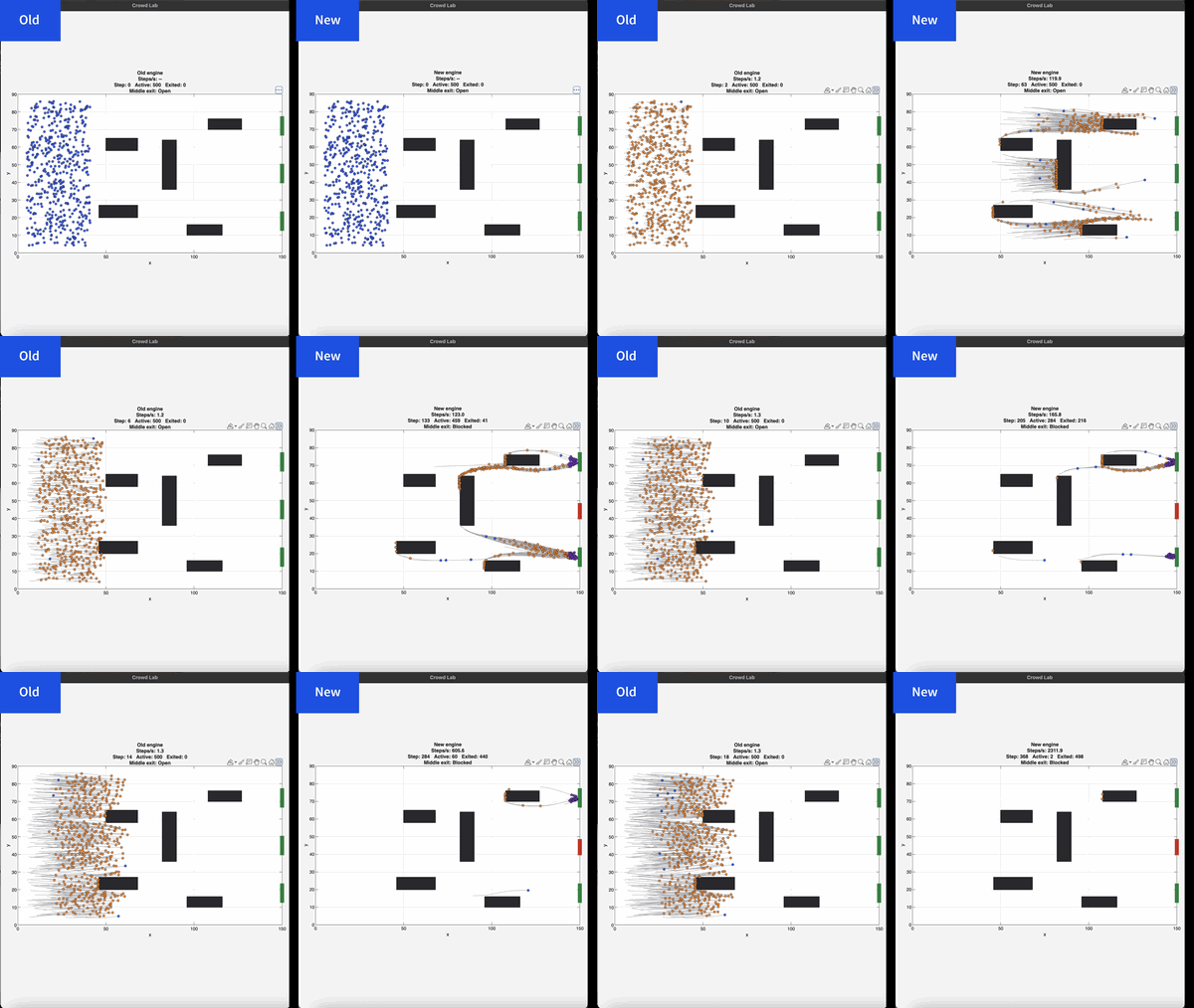
If you prefer numbers to pictures, all of the details are in a blog post from when we released the limited beta: Objects are about to get much faster in MATLAB » The MATLAB Blog - MATLAB & Simulink
"Why didn't we make this the default?" I hear you ponder. Because there is a small chance that the new system will break your code. It's a very small chance and I've personally not seen any code that does get broken. However, such code does exist and we want to be give you the chance to discover this and work with us to make your code compatibile before it does become the default.
I hope you enjoy using 2026b as much as we enjoyed making it.
Cheers,
Mike
I keep forgetting the functions and lack of pratices would be the reason

Extremely--I have real work to do
24%
Maybe talk about something else?
24%
Neutral
24%
Not very much
24%
Let's talk about nothing else
5%
21 votos

This Week's Quiz
119 responses

Hey, this is a safe space to share your cool projects you know. I have pet ducks, I use ThingSpeak to open the door to their house each morning. I just finished an upgrade to the LED strip lights on my driveway that are controlled via ThingSpeak. And the valves for my drip irrigation system. You got it. Controlled by ThingSpeak. Let me know your last cool project you finished or the one you keep dreaming of starting. I need some more inspiration :)

I contributed a guet post for @Mike Croucher - AI Agent Demystified – Building a Minimalist Agent in MATLAB
Basically, my use case is an coding agent built with MATLAB to code MALTAB, but you can actually roll your own agnet with MATLAB AI Agent SDK for more realistic use cases. Hopefully my post gives you a starting point for a fun exploration!

The example code below shows how to write version 7.3 MAT files directly from C++ using the HDF5 library (libhdf5) and HighFive, a header-only C++ wrapper for libhdf5. Version 7.3 MAT files are HDF5-based, but contain a proprietary header in the first 512 bytes of the file.
The implementation performs three primary tasks:
First, it creates an HDF5 file with a 512-byte userblock. After data has been added into the file, the file is closed. Then a 128-byte header is written into the userblock so that the file is recognized by MATLAB as a valid version-7.3 MAT file. This is done in function “makeMatHeader”.
Second, MATLAB-specific metadata attributes are added to each dataset. Attributes such as “MATLAB_class” and “MATLAB_int_decode” inform MATLAB how each dataset should be interpreted.
Third, MATLAB-compatible complex datasets are created by overriding HighFive's default complex-number layout. HighFive uses the field names `r` and `i` by default, while MATLAB expects `real` and `imag`. A Highfive custom compound type is therefore registered for `std::complex<double>` using the MATLAB field names.
With these changes in place, C++ code can write scalar values, vectors, structs, complex arrays, and character arrays to a file that MATLAB can read as a version 7.3 MAT file.
#include <iostream>
#include <vector>
#include <complex>
#include <cstddef>
#include <fstream>
#include <string>
#include <cstdint>
#include <utility>
#include <bitset>
#include <highfive/highfive.hpp>
#include "hdf5.h"
// Modify the 512-byte userblock at the front of the HDF5 file to make it compatible with MATLAB's v7.3 MAT file format.
void makeMatHeader(std::string filename)
{
char header[512]; // MATLAB-style header for HDF5 file
memset(header, 0, sizeof(header)); // Initialize header to all zeros
// Example header content
snprintf(header, sizeof(header), "MATLAB 7.3 MAT-file, Platform: HDF5");
header[124] = 0;
header[125] = 2;
// I/M indicate little-endian format (Intel Mac/Windows)
header[126] = 'I';
header[127] = 'M';
// Write the header to the beginning of the file
std::ofstream outFile(filename, std::ios::binary | std::ios::in | std::ios::out);
outFile.seekp(0);
outFile.write(header, sizeof(header));
outFile.close();
}
// https://www.geeksforgeeks.org/dsa/inplace-m-x-n-size-matrix-transpose/
void MatrixInplaceTranspose(int *A, int rows, int cols)
{
// Moves elements in-place to achieve the transpose.
// A is a pointer to a 2D array, rows is the number of rows, and cols is the number of columns.
int size = rows*cols - 1;
int t; // holds element to be replaced, eventually becomes next element to move
int next; // location of 't' to be moved
int cycleBegin; // holds start of cycle
int i; // iterator
const int HASH_SIZE = 8192; // define a suitable hash size for the bitset. Must be at least as large as the number of elements in the matrix.
std::bitset<HASH_SIZE> b; // hash to mark moved elements. Must be large enough to cover all indices.
if (rows <= 0 || cols <= 0) {
throw std::invalid_argument("Matrix dimensions must be positive");
}
else if ((rows * cols) > HASH_SIZE)
{
throw std::invalid_argument("Matrix size exceeds hash size for in-place transpose. Increase the HASH_SIZE constant.");
}
b.reset();
b[0] = b[size] = 1;
i = 1; // Note that A[0] and A[size-1] won't move
while (i < size)
{
cycleBegin = i;
t = A[i];
do
{
// Input matrix [rows x cols]
// Output matrix [cols x rows]
// i_new = (i*rows)%(N-1)
next = (i*rows)%size;
std::swap(A[next], t);
b[i] = 1;
i = next;
}
while (i != cycleBegin);
// Get Next Move (what about querying random location?)
for (i = 1; (i < size) && b[i]; i++)
;
}
}
template <typename T>
std::vector<std::vector<T>> transpose(const std::vector<std::vector<T>>& matrix)
{
// Performs a nonconjugate transpose on a vector of vectors
// The input matrix is a vector of vectors, where each inner vector represents a row of the matrix.
// Handle empty matrix edge case
if (matrix.empty() || matrix[0].empty()) {
return {};
}
size_t rows = matrix.size();
size_t cols = matrix[0].size();
// Initialize the transposed matrix with flipped dimensions: cols x rows
std::vector<std::vector<T>> transposed(cols, std::vector<T>(rows));
for (size_t i = 0; i < rows; ++i) {
for (size_t j = 0; j < cols; ++j) {
transposed[j][i] = matrix[i][j];
}
}
return transposed;
}
// Creates a HighFive compound type for representing MATLAB-style complex numbers
// HighFive by default uses r/i but that is not compatible with MATLAB's complex number representation, which uses real/imag.
HighFive::CompoundType matlabComplexDouble () {
return {
{"real", HighFive::AtomicType<double>{}},
{"imag", HighFive::AtomicType<double>{}}
};
}
// Register the CompoundType to represent std::complex<double>
HIGHFIVE_REGISTER_TYPE(std::complex<double>, matlabComplexDouble);
int main()
{
const std::string filename = "test.mat";
// Needed for the complex number literal suffix 'i'
using namespace std::literals;
/*
* MATLAB vs C++ array layout
*
* MATLAB stores arrays in column-major order, meaning values in the same column are
* laid out next to each other in memory. Typical C++ containers such as nested std::vector and arrays
* are written in row-major order, where values in the same row are adjacent in memory.
*
* That difference matters when something such as a 2D dataset is exchanged from C++ to MATLAB. A 2x3
* matrix written from C++ in row-major order will be interpreted by MATLAB as a 3x2 matrix, transposed relative
* to the original C++ layout. The user will have to transpose the array to view the original C++ layout
* correctly.
*
* C++ developers need to be aware of the memory layout when
* exchanging multidimensional arrays with MATLAB. To maintain the structure,
* one will need to transpose the array before writing it to the mat file.
*/
// Test data
// 2x3 Array of complex double
std::vector<std::vector<std::complex<double>>> dataComplex = {{10.0 + 1.0i, 20.0 + 2.0i, 30.0 + 3.0i},
{40.0 + 4.0i, 50.0 + 5.0i, 60.0 + 6.0i}};
// 1x3 Vector of double
std::vector<double> dataDoubleVec = {1.1, 2.2, 3.3};
// 1x5 Array of integers
int dataIntArray[5] = {1, 2, 3, 4, 5};
// 2x4 Array of integers
int dataIntArray2x4[2][4] = {{1, 2, 3, 4},
{5, 6, 7, 8}};
int dataInt = 79;
double dataDouble = 3.14;
std::string dataString = "Hello, MATLAB!!!!!";
{
// Put the highfive related code into its own block so that the file gets closed when the file object is no longer in scope.
// Create a highfive file create property, get the underlying HDF5 property ID, and set a userblock size
HighFive::FileCreateProps fcp = HighFive::FileCreateProps::Empty();
hid_t fcpl_id = fcp.getId();
H5Pset_userblock(fcpl_id, 512);
HighFive::File file(filename, HighFive::File::Truncate, fcp);
// Storing a double to the file
// For something that is only a single value, must create a 1x1 dataspace
HighFive::DataSpace scalarDoubleSpace({1, 1});
// This creates a variable in the MATLAB workspace with the name "double_value"
HighFive::DataSet doubleField = file.createDataSet<double>("double_value", scalarDoubleSpace);
doubleField.write(dataDouble);
// Metadata for MATLAB compatibility
doubleField.createAttribute("MATLAB_class", std::string("double"));
// Storing an integer to the file
// For something that is only a single value, must create a 1x1 dataspace
HighFive::DataSpace scalarIntSpace({1, 1});
// This creates a variable in the MATLAB workspace with the name "int_value"
HighFive::DataSet intField = file.createDataSet<int>("int_value", scalarIntSpace);
intField.write(dataInt);
// Metadata for MATLAB compatibility
intField.createAttribute("MATLAB_class", std::string("int32"));
// Storing a C-style 1x5 array of integers to the file
// Since it is a single dimension, there is no need to move the data, just reinterpret it as a 5x1 row-major array.
// When Matlab imports it, it will perceive it as a 1x5 column-major array.
// This line casts the 1x5 array to a 5x1 array to match MATLAB's column-major order
int (*numArrayTrans5x1)[1] = reinterpret_cast<int (*)[1]>(dataIntArray);
HighFive::DataSpace intArray5x1Space({5, 1});
// This creates a variable in the MATLAB workspace with the name "int_array"
HighFive::DataSet intArrayField = file.createDataSet<int>("int_array", intArray5x1Space);
intArrayField.write(numArrayTrans5x1);
intArrayField.createAttribute("MATLAB_class", std::string("int32"));
// Storing a C-style 2x4 array of integers to the file
// For something that is a multi-dimensional array, we need to transpose the array and create a dataspace with the dimensions swapped
// so that the data is stored in column-major order.
MatrixInplaceTranspose((int*)dataIntArray2x4, 2, 4);
// After moving the values around, we need to cast the array with the new dimensions to match the new layout
// Cast the transposed 2x4 array to a 4x2 array to match MATLAB's column-major order
int (*numArrayTrans)[2] = reinterpret_cast<int (*)[2]>(dataIntArray2x4);
HighFive::DataSpace intArray2x4Space({4, 2});
// This creates a variable in the MATLAB workspace with the name "int_array_2x4"
HighFive::DataSet intArray2x4Field = file.createDataSet<int>("int_array_2x4", intArray2x4Space);
intArray2x4Field.write(numArrayTrans);
intArray2x4Field.createAttribute("MATLAB_class", std::string("int32"));
// Creating a Matlab struct (HDF5 group)
HighFive::Group my_struct = file.createGroup("my_struct");
my_struct.createAttribute("MATLAB_class", std::string("struct"));
// The only difference between storing data into a struct or as a normal variable in the MAT file is the
// the parent object you use when you do "createDataSet".
// file.createDataSet would create a normal variable, my_struct.createDataSet creates it within the "my_struct" struct.
// Storing a string to the struct so that it will be accessible as a character array in MATLAB
// For something that is a string, we create a dataspace with dimensions [string_length, 1] and save the character data accordingly
// We create a vector that has dataString.size() elements, each of which is a char vector of size 1 to store individual characters.
std::vector<std::vector<char>> text_bytes(dataString.size(), std::vector<char>(1));
// MATLAB expects character arrays to be a row vector so we reshape it accordingly since dimensions are swapped between C++ and MATLAB
for (int i = 0; i < dataString.size(); ++i) {
text_bytes[i][0] = dataString[i];
}
HighFive::DataSpace charSpace({dataString.size(), 1});
// uint16_t is required for MATLAB character arrays
HighFive::DataSet textField = my_struct.createDataSet<uint16_t>("text_value", charSpace);
textField.write(text_bytes);
// Metadata for MATLAB compatibility
textField.createAttribute("MATLAB_class", std::string("char"));
// Tell MATLAB to interpret the data as characters rather than integers
textField.createAttribute("MATLAB_int_decode", 2);
// Storing a vector to the struct
// In order to transpose the vector correctly, we first wrap it in another vector to make it a 2D array.
std::vector<std::vector<double>> transposableDoubleVec = { dataDoubleVec };
// For vectors, we let HighFive infer the dataspace from the data itself
// Transpose the vector to match MATLAB's column-major order
HighFive::DataSet doubleVectorField = my_struct.createDataSet("double_vector", transpose(transposableDoubleVec));
// Metadata for MATLAB compatibility
doubleVectorField.createAttribute("MATLAB_class", std::string("double"));
// Storing a complex (and multi-dimensional) vector to the struct
// For multi-dimensional vectors, we need to perform a noncojugate transpose on the array to match
// MATLAB's column-major order so the data layout is consistent between C++ and MATLAB.
// For vectors, we let HighFive infer the dataspace from the data itself
HighFive::DataSet complexField = my_struct.createDataSet("complex_vector", transpose(dataComplex));
// Metadata for MATLAB compatibility
complexField.createAttribute("MATLAB_class", std::string("complex"));
}
// Finalize the MATLAB-compatible HDF5 file by writing the MATLAB header into the userblock
makeMatHeader(filename);
return 0;
}
Looking for a quick way to test your MATLAB knowledge and learn something new?
Starting today, we're launching Weekly Quizzes in Discussions. Each week, you'll find one multiple-choice question designed to challenge your MATLAB knowledge, spark curiosity, or teach you something new. Most quizzes take only a few minutes to complete, and after you solve, you can view the explanation, hints, or study guide provided by the quiz creator.
- New quiz every week
- No coding required
- Learn something new in minutes
- Build your participation streak
Ready for this week's challenge?
⚠️ Fair warning: It's trickier than it looks. I got it wrong. How about you?

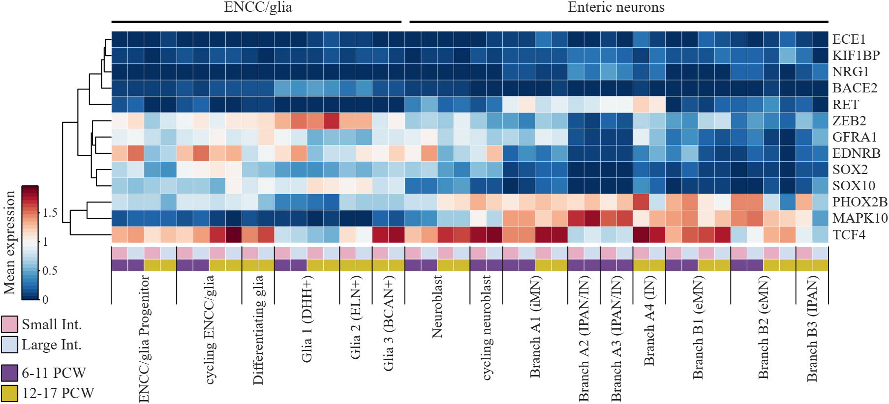
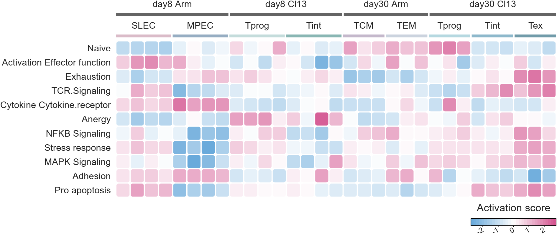
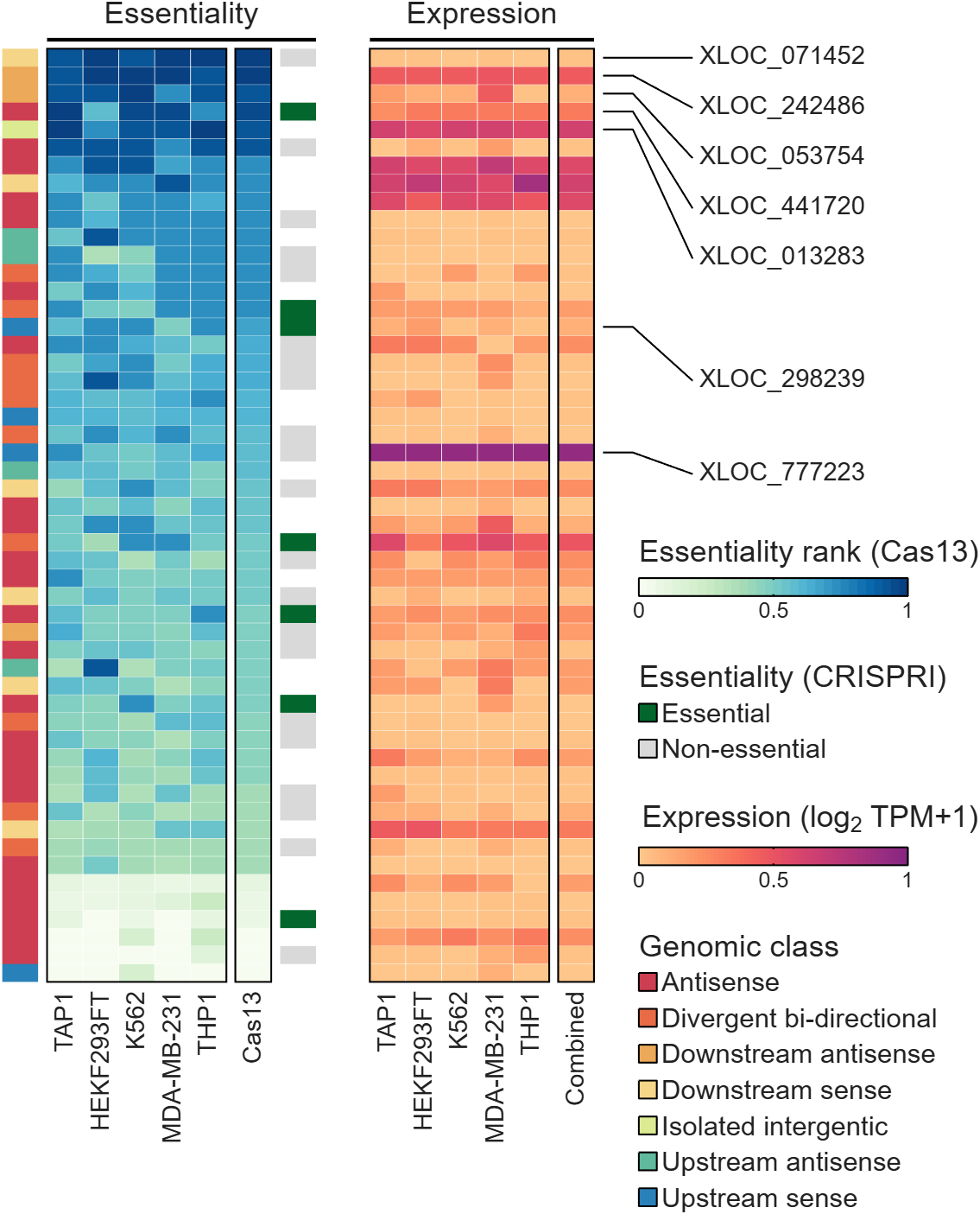
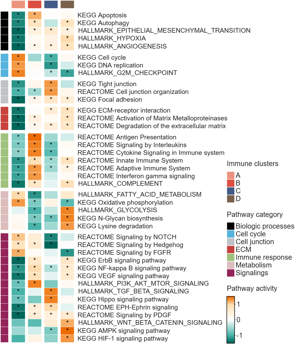
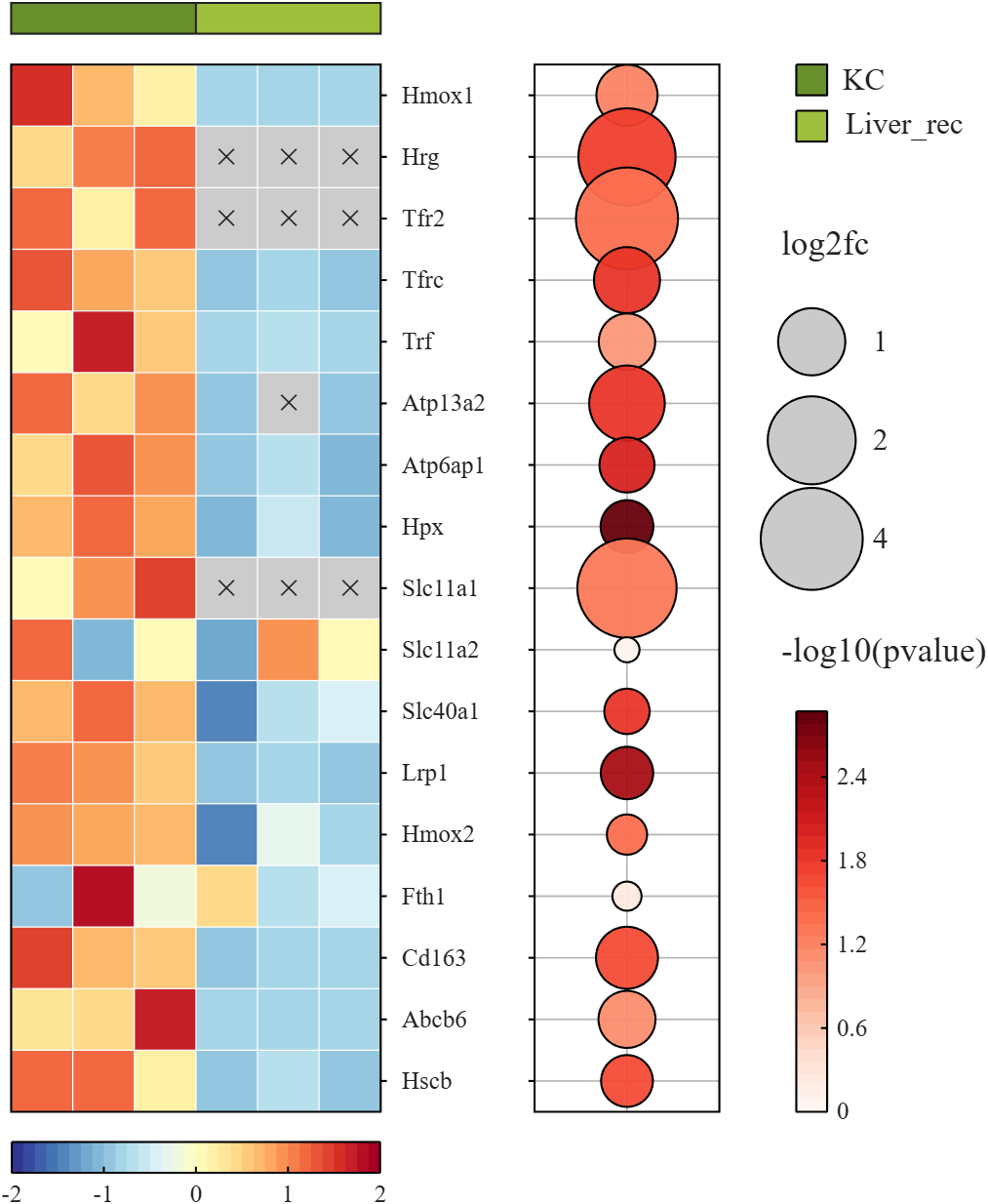
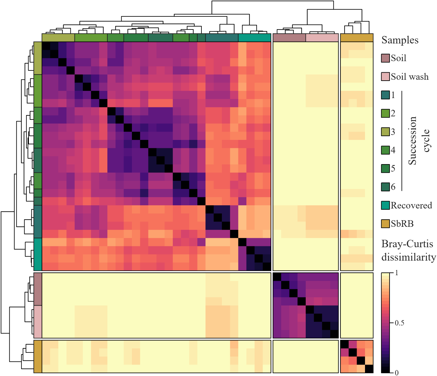
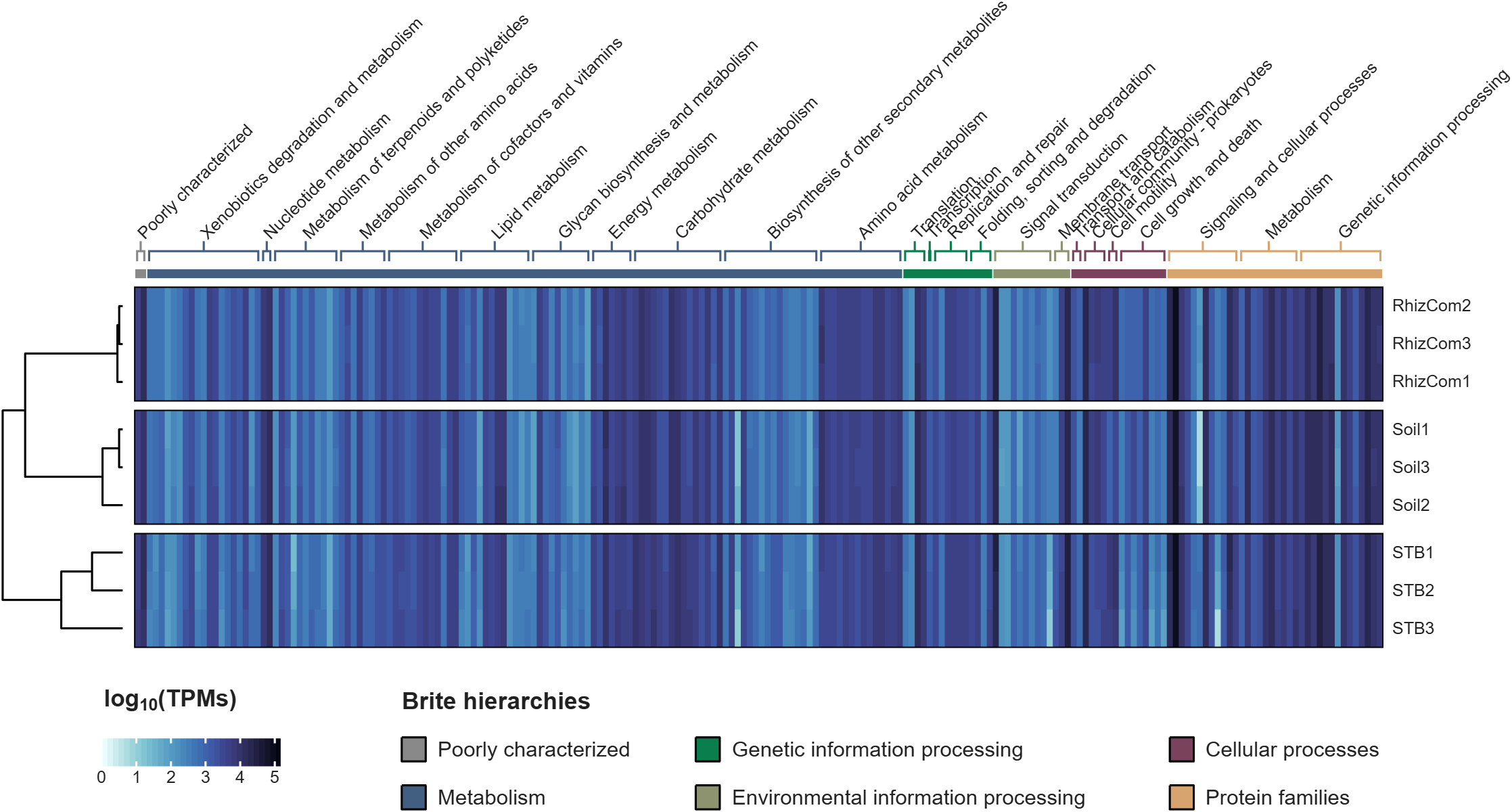
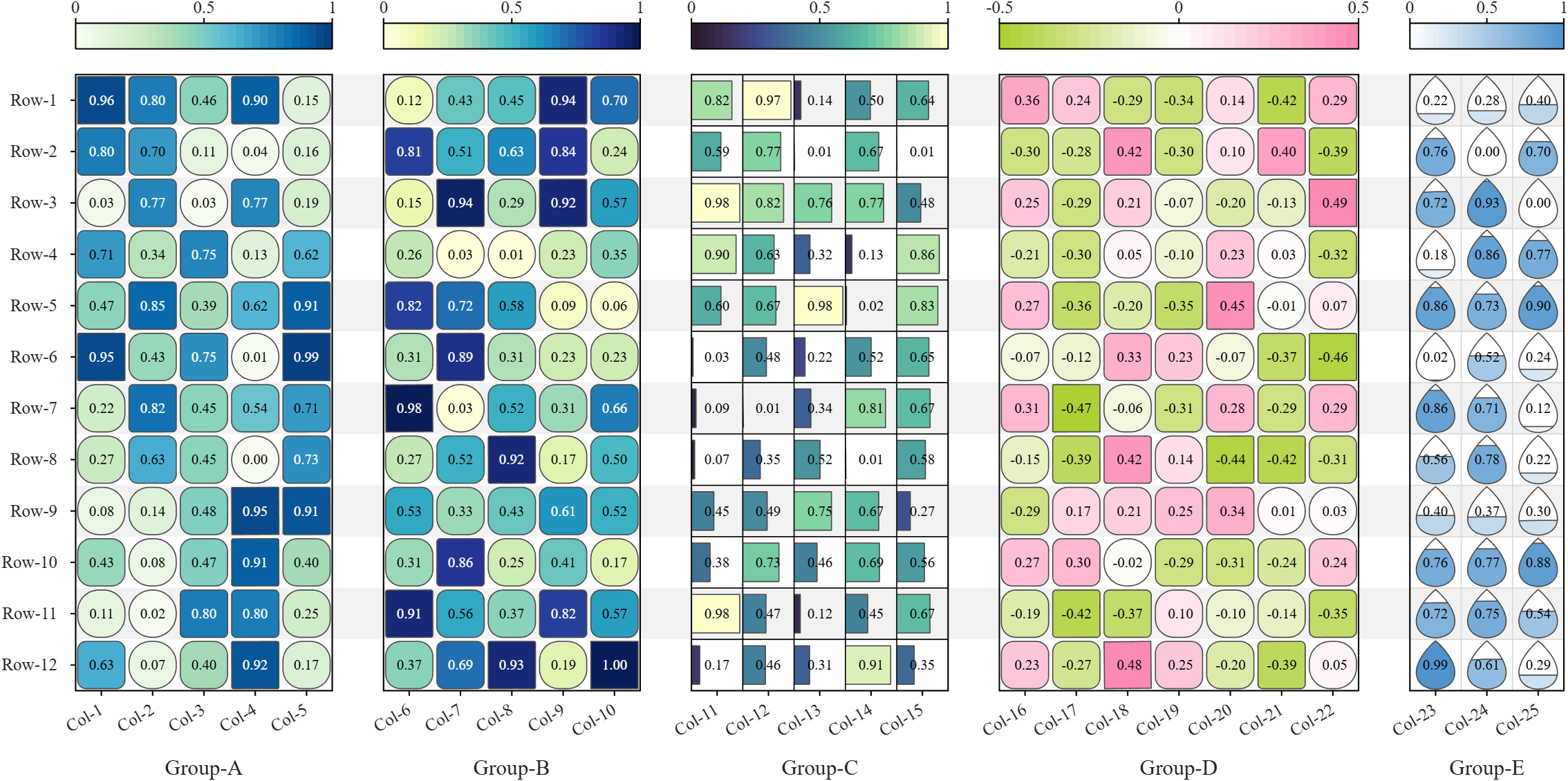
All these examples are plotted using SHeatmap. For details, please refer to the relevant examples in the demo_SColorbar folder included in the toolbox.

Claudifying MATLAB
Duncan Carlsmith
Department of Physics, University of Wisconsin-Madison

Introduction
AI mobile and desktop apps are convenient interfaces for exploration. For programmatic work not subject to variations in AI response, an AI can generate standalone code and web workflows. (See e.g. Web Automation with Claude, MATLAB, Chromium, and Playwright.) Intermediate is your own code that can batch process input data with AI via API.
Large Language Models (LLMs) with MATLAB permits a script to connect to OpenAI Chat Completions and Images, Azure OpenAI, Ollama, and other services that accept the OpenAI format. This submission introduces an educational Live Script Claude API from MATLAB for Coursework that illustrates how to access Anthropic models via API with MATLAB, using example tasks relevant to physics education, and might be adapted for other AI vendor APIs or emulated for other applications. This submission is essentially the Live Script introduction.
The script lists the available Claude models, sends text, images, and PDFs to a chosen model, holds a multi-turn conversation, extracts structured data from a document, lets Claude call MATLAB functions, and grades a set of short answers against a rubric. The examples show how an instructor or a student might use an AI model as a programmable assistant, for feedback on a figure, a check of a lab report, or a first pass at grading.
The Messages API is a web service at https://api.anthropic.com/v1/messages. A program sends it a request in JSON, the text format used for structured data on the web, and receives Claude's reply in JSON. A request names a model, sets a limit on the length of the reply, and carries a list of messages. An optional system prompt holds standing instructions that apply to every turn. The service keeps no memory between requests, so each request carries the whole conversation so far. MATLAB builds each request as a struct and jsonencode converts it to JSON.
Lengths and prices are counted in tokens. A token is a fragment of text, on average about four characters of English. Each response reports how many input and output tokens it used.
Helper functions in this folder handle the web requests and the bookkeeping. claudeRequest sends one request and reports the server's error message on failure. claudeListModels returns the models available to the key. claudeConversation and askClaude hold a multi-turn conversation and add up tokens and cost. claudeImageBlock and claudePdfBlock package a file for a message, claudeText extracts the reply text, and claudeCost converts token counts to dollars.
The example inputs sit in the inputs folder, which the Python version shares, and are fictional. example_flawed_figure.png is a plot with deliberate defects. example_lab_report.pdf is a student lab report with three planted errors, and example_lab_report_page1.png is an image of its page for display. student_answers.csv holds five short answers of varying quality. Output files go to the matlab_outputs folder and carry a timestamp in the name, so no run overwrites an earlier one, and the MATLAB and Python outputs stay apart.
"Try this" blocks mark the settings to change. The references list the API documentation. The appendix on privacy and security describes where requests go, how long the vendor keeps them, and precautions for student work and for the API key. A parallel Python version of the script and helper functions is in the Python folder. These functions could be called from MATLAB or invoked from a terminal.
Acknowledgments and disclaimer
The author has no financial interest in any company or product named here. Nothing in this post is endorsed by, sponsored by, or an official position of the University of Wisconsin-Madison.

