Resultados de
The stationary solutions of the Klein-Gordon equation refer to solutions that are time-independent, meaning they remain constant over time. For the non-linear Klein-Gordon equation you are discussing:
Stationary solutions arise when the time derivative term,  , is zero, meaning the motion of the system does not change over time. This leads to a static differential equation:
, is zero, meaning the motion of the system does not change over time. This leads to a static differential equation:This equation describes how particles in the lattice interact with each other and how non-linearity affects the steady state of the system.
The solutions to this equation correspond to the various possible stable equilibrium states of the system, where each represents different static distribution patterns of displacements  . The specific form of these stationary solutions depends on the system parameters, such as κ , ω, and β , as well as the initial and boundary conditions of the problem.
To find these solutions in a more specific form, one might need to solve the equation using analytical or numerical methods, considering the different cases that could arise in such a non-linear system.
By interpreting the equation in this way, we can relate the dynamics described by the discrete Klein - Gordon equation to the behavior of DNA molecules within a biological system . This analogy allows us to understand the behavior of DNA in terms of concepts from physics and mathematical modeling .
% Parameters
numBases = 100; % Number of spatial points
omegaD = 0.2; % Common parameter for the equation
% Preallocate the array for the function handles
equations = cell(numBases, 1);
% Initial guess for the solution
initialGuess = 0.01 * ones(numBases, 1);
% Parameter sets for kappa and beta
paramSets = [0.1, 0.05; 0.5, 0.05; 0.1, 0.2];
% Prepare figure for subplot
figure;
set(gcf, 'Position', [100, 100, 1200, 400]); % Set figure size
% Newton-Raphson method parameters
maxIterations = 1000;
tolerance = 1e-10;
% Set options for fsolve to use the 'levenberg-marquardt' algorithm
options = optimoptions('fsolve', 'Algorithm', 'levenberg-marquardt', 'MaxIterations', maxIterations, 'FunctionTolerance', tolerance);
for i = 1:size(paramSets, 1)
kappa = paramSets(i, 1);
beta = paramSets(i, 2);
% Define the equations using a function
for n = 2:numBases-1
equations{n} = @(x) -kappa * (x(n+1) - 2 * x(n) + x(n-1)) - omegaD^2 * (x(n) - beta * x(n)^3);
end
% Boundary conditions with specified fixed values
someFixedValue1 = 10; % Replace with actual value if needed
someFixedValue2 = 10; % Replace with actual value if needed
equations{1} = @(x) x(1) - someFixedValue1;
equations{numBases} = @(x) x(numBases) - someFixedValue2;
% Combine all equations into a single function
F = @(x) cell2mat(cellfun(@(f) f(x), equations, 'UniformOutput', false));
% Solve the system of equations using fsolve with the specified options
x_solution = fsolve(F, initialGuess, options);
norm(F(x_solution))
% Plot the solution in a subplot
subplot(1, 3, i);
plot(x_solution, 'o-', 'LineWidth', 2);
grid on;
xlabel('n', 'FontSize', 12);
ylabel('x[n]', 'FontSize', 12);
title(sprintf('\\kappa = %.2f, \\beta = %.2f', kappa, beta), 'FontSize', 14);
end
% Improve overall aesthetics
sgtitle('Stationary States for Different \kappa and \beta Values', 'FontSize', 16); % Super title for the figure
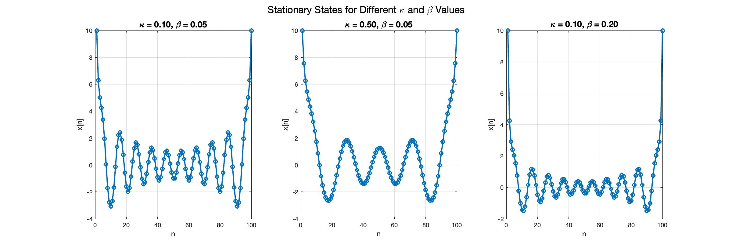
In the second plot, the elasticity constant κis increased to 0.5, representing a system with greater stiffness . This parameter influences how resistant the system is to deformation, implying that a higher κ makes the system more resilient to changes . By increasing κ, we are essentially tightening the interactions between adjacent units in the model, which could represent, for instance, stronger bonding forces in a physical or biological system .
In the third plot the nonlinearity coefficient β is increased to 0.2 . This adjustment enhances the nonlinear interactions within the system, which can lead to more complex dynamic behaviors, especially in systems exhibiting bifurcations or chaos under certain conditions .