System-level Simulation of an Aperture Array Beamformer
Kaushal Buch, Giant Metrewave Radio Telescope, NCRA-TIFR
Sreekar Sai Ranganathan, Indian Institute of Technology Madras
A multi-element, multi-beam aperture array beamforming system is being developed as part of the Expanded GMRT (eGMRT) project. This prototype system is a part of the proposal aimed at improving the scientific capabilities of the Giant Metrewave Radio Telescope (GMRT), one of the most sensitive instruments in the world for observing celestial objects at meter-wave radio frequencies. The initial prototype beamforming system built on an FPGA and operating in the L-band (1.1-1.7 GHz) is undergoing testing in a free-space test range at the GMRT site. In parallel with the efforts towards the final prototype development, we carried out an end-to-end simulation of the beamforming system by modeling the Vivaldi antenna array, RF and analog signal processing systems, and digital beamformer using MATLAB® and Simulink®. The free-space testing was simulated by modeling the transmitting antenna, propagation channel, and sources of interference for testing multiple beams. The simulation was carried out in Simulink using multiple toolboxes for the beamformer's accurate modeling, including the antenna array, test range, and array signal processing algorithms. We tested phased array beamsteering, nulling, and maxSNR beamforming algorithms/techniques for linear and rectangular arrays in the simulation and compared them with the experimental results. We kept the model parameters for the beamforming system simulator similar to those in the actual system. This enabled us to see the difference in the performance of actual and simulated systems. Optimal beamforming was simulated in a case with mutual coupling between the antenna elements to understand its effect on the array covariance matrix, signal-to-noise ratio, and the array calibration process. This presentation would describe the simulator architecture and various beamforming tests and compare the results with the actual system performance. The simulator has a workflow-based framework to encapsulate future requirements of the project and to support diverse array signal processing and beamforming applications.
Published: 25 May 2022
[MUSIC PLAYING]
Hello. I am Kaushal Buch. I work as an engineer with the digital backend group at the Giant Meteorological Telescope, which is located in Pune, India. Along with me, I have to co-authors, Sreekar Ranganathan, who is a student working with me on this project, and Bela Dixit, who is a colleague at GMRT. We're here to talk about system-level simulation of an aperture array beamformer.
So the agenda of the talk would be aperture arrays in astronomy, challenges in aperture array beamformer simulation, and end-to-end simulation framework, testing and benchmarking of the simulation model. And finally, we'll summarize the results and findings in the concluding slides.
So what are aperture arrays? So aperture arrays are array of antennas, elements which have an associated RF, analog, and digital signal processing system. They are basically used for beamforming and spatial filtering. The typical applications are in communication, engineering, array signal processing, radar signal processing, and most recently, in radio astronomy.
Now, there are a few challenges associated with these kind of aperture arrays. So when you beamform these arrays, you need to calibrate the presence of mutual coupling. And then the signal processing becomes complicated because of more number of elements and wider bandwidth.
So on the bottom, one can see the Vivaldi element. So these are the Vivaldi elements. And they are arranged in horizontal and vertical polarization. These are individual elements. And then one could see a kind of eight across line array of Vivaldi elements, to polarizations, which makes it a 144 element Vivaldi element array in L band put into a cavity. So this is a typical kind of antenna array which you will see.
So how are aperture arrays important to radio astronomy? So radio astronomy is done through instruments called radio telescopes, which detect radio emissions coming from stellar objects. So these are very faint emissions. So certainly, you need a very sensitive receiver to pick this up and do science out of these data. So aperture arrays provide a wider field of view.
Generally, the radio telescope antennas are wider in diameter to get more collecting area, which restricts their field of view. The use of aperture array improves the field of view while giving a similar sensitivity, and one could do a large number of survey of celestial objects while observing the sky. So we get a wider field of view and increased survey speed and a better sensitivity.
Some examples of aperture arrays. So this is a one called the Low Frequency Array, located in Europe, in Netherlands. And these are the tiles which have the elements, and the associated processing is done at a central location. And these are the ones used to survey the sky at radio frequencies.
Similarly, if the array is mounted on the focal plane of a dish, then they are known as focal plane arrays, or faced array feeds So here you can see on the right, you could see such an example where the aperture array is mounted on the field.
Now, this image tells you-- uses a general idea about where these aperture arrays, what are the various applications of aperture arrays in radio astronomy. So one of the things which we saw in the previous slide was that it increases the field of view, and it allows possibilities of surveying the sky in different dimensions, in different spatial dimensions.
So one could see here that there are beams pointing at different locations in the sky, and one could sort of get signals from galaxies, pulsars, and various other sources in the sky, astronomical sources in the sky, in the universe. And at the same time, the advantage is that one could also form nulls in the direction of interference. So one could see here that there is a satellite, and another could be formed here. So this is an extraterrestrial source of interference. Similarly, a terrestrial source of interference, like a cell phone tower, the interference from these kind of things can be mitigated by shaping the beam in a proper manner. So now let's talk about the expanded GMRT project, the aperture array development in that, and how this simulation helped in understanding the various aspects of aperture array beamforming.
So GMRT is a radio telescope located in India. It's one of the most sensitive instruments at low radio frequencies. And the expansion of GMRT has one of the elements proposed, which will look at the aperture array of focal plane array development. So here we have a 144 element Vivaldi, the one which I showed in the earlier slide, which has an integrated [INAUDIBLE] amplifier, which feeds the signal to the optical transmitter module, which sends the data over the optical fiber to a central location where it is downconverted it is digitized and then we have a digital beamformer on FPGA which can produce a 32-element input. It can produce of 5-beam output with a 32-element input. And the data is acquired using a computer.
So what do you mean by aperture array beamformer simulation, and what does it require? So a typical simplified block diagram of a two-element beam format has antenna elements at its input, which convert the electromagnetic signal into electrical signal. This signal needs to be amplified, at times downconverted, depending on the kind of receiver system, digitized, and the rest of the processing beamforming happens in the digital domain, mostly in the frequency domain.
So this digitized signal is Fourier transformed into frequency domain signal, and beamforming is done by multiplying different weights. And these are complex weights, amplitude and phase. So how do you get the weights? So the weights are calculated from something called the correlator which correlates the signal coming from two antennas, and it used the amplitude and phase for correcting and combining the signals in the right manner in this beam beamformer output. So if you have two beams, you need to get two different sets of amplitude and phase for multiplying the weights.
So this is how you form a multibeam system. And here, we have used antenna and phased array toolbox for modeling the antenna element pattern. You have used the RF and antenna toolbox for modeling the receiver gain of variations and mutual coupling. And we have used signal processing toolbox similarly, and in general, the Matlab for modeling the hardware imperfections that we see on the FPGA or finite arithmetic which we see on FPGA, and model it into the simulated environment.
So now the way we test this initially while we develop the aperture array, the method which we have used is that at the GMRT site, we have a transmitting dish, a 3-meter dish antenna. And on the other end of the building, we have the aperture array, or the focal plane array, under test, which one can see here. And this is an L band radiation test range. So the distance is about 67 meters, which is the far field for a 3-meter diameter antenna. And this is how we test. So there are certainly a lot of reflections in this test range, which we'll model, which we'll see, and which we will also account for in the simulation part.
So what are the major components of the simulation model? So as we now saw that we have a transmitting antenna, a propagation channel, a receiving antenna, and then the receiving signal processing system. So first, we need to model a parabolic reflector similar to the one which we have in the test range, which is a 3-meter parabolic dish. So we use various Antenna Toolbox elements. One of them was the reflector parabolic feature.
Then in the simulation, the next step would be to have a receiver antenna array, which would have the Vivaldi, which is similar to the one which we have at the site, which we are using for various of our experiments. And here we have used various antenna element features. One of them is the egg crate feature, which is a very recent addition.
And then finally, we need to simulate the RF systems, where we can have the gain and phase variations, where we can add the mutual coupling between the elements. And then finally, the digital beamformer, which will digitize the signal, Fourier transform it, multiply it, multiply the weights, and then combine the signal to get the desired beam output.
So let's go to modeling the Vivaldi antenna array. Now, one of the examples of this is given in this snippet of code here, where we use the Vivaldi offset cavity. And what the method which we have chosen for system level simulation is to model one Vivaldi element, like the one which is shown here as an example. This is the radiation pattern of a Vivaldi with an infinite ground plane, and at 1.3 gigahertz.
And individual element patterns are modeled in this way. And then we have an Excel sheet with which we can select the array geometry. So here you can see, we have chosen a 4 cross 4 array, which is a rectangular array, uniform rectangular array.
So what this does in the background is it used the dimension of the array. It used the xyz coordinates of the array so that one can model the phase delay or the path difference between the elements while we simulate this system. The mutual coupling is, in our case, for system simulation we add the mutual coupling later on in the receiver system.
So how do we add mutual coupling? So mutual coupling can be derived from the impedance parameters of the array. So we introduce it after we get the individual element pattern. We get a matrix of coupling values, and we multiply that with the incoming data. So if you see here, this is a simulated block where we take the transpose and we multiply the coupling matrix. And just to make the data as it was before, we take another transpose. And the effect can be seen in the cross correlation.
So if there is a coupling, it'll show up as a power, which is coupled in the adjacent elements. So if you see this cross correlation matrix over here for 8 cross 1 uniform linear array, so on the diagonal, you have the autocorrelation. So the normalized cross correlation is 1. It is correlated with itself.
Now, if you see the elements which are adjacent, you would see a coupling of 0.2, 0.3. So that is 10%, 20% kind of coupling. And these are all values generated by changing the parameters of this coupling. So this is just an example showing how the coupling would show up in the cross correlation.
Now, one of the important things when we design any facility is the calibration part, right? So one needs to know the amplitude and phase correctly for each element and then correct for it to make a coherent beam or to apply appropriate weights.
So here we have in order to generate and to check what is the effect of gain and phase fluctuations variations in the analog chain on the calibration path, we generate a randomized gain by a multiplying factor within a certain range specified, which is user specific, and a phase shift, which is done by the RF phase shifters, which is also user specific. And this, within that range of user specified values, it picks up a uniformly random number and multiplies it with that number.
And again, here now this time, this is a correlation matrix, but slightly of a different kind. So this is an 8-element, again, 8 cross 1 uniform linear array correlation matrix, but this is a full spectrum matrix. So these are the channels over here, all the channels in the box you can see here, where the cursor is pointing.
So this half, the lower triangle, is the amplitude. That's the magnitude spectrum. And the upper triangular matrix is the phase spectrum. So you can see here on both the sides, the color bar, and you can see that the values are randomized. This is one such instance to show how randomization is tested.
Now, coming to the entire system simulation model at a top level, we have to radiate a certain signal. So we can either radiate a tone signal a single frequency signal or broadband noise and then this one can radiate and give it to the transmit array, which is actually a parabolic reflector in our case. That one has a propagation model.
So here you have the ability to introduce multiple transmitters to see if one can do special filtering and mitigate interference, et cetera. Then this goes to the receiver array, which is a Vivaldi element array. Then we have the coupling model and randomizing the gain and phase of the system, then taking the Fourier transform, and then the correlator part, which used the amplitude and phase values for the weights. Then we calculate the weights externally and then feed those values to the beamformer. This is beam 1 and beam 2, with different weights. And all of this is orchestrated through a Matlab script which decides the configuration parameters of each of the blocks. And also, the output data is processed and get the desired plots.
So end-to-end system-level simulation, you start by programming the different values in the simulation model. First, you record the correlation data. That is, you calibrate the array. You get the data as required, then you calculate the weights. So this example is for beam steering. So you calculate the weights for the coherent beam. So basically, you correct the differences of phase and amplitude between the elements to form a phased array beam or a coherent beam.
Then you run the beamformer part of it, generate a beam angle corresponding to a steering angle, generate the beamformer spectrum, and repeat this for all the angles. And that's where you get the beam intensity as a function of steering angle.
So if you see here, we have two examples. One is beam steering from minus 60 degrees to plus 60 degrees for a single-- this is broadband noise radiation. In the simulation model, we have enabled broadband noise radiate array passed to the propagation channel. And here you can see that we have a beam pattern at every 4 degrees [INAUDIBLE] size. And one could see that since it was a rectangular window, you can see the side look level at minus 13 dB. The beam width for a 1 meter array, 8 cross 1 uniform linear array, should be around 13 degrees. It is coming close to 12.65. And this is at 1.3 gigahertz, OK?
Now, this is the figure on the left. Now, the figure on the right shows how we tested multi-beamforming. So one of the ways in which one can check multi-beamforming is by steering the null at the boresight. So you have one beam which is a phased array beam, a coherent beam at the boresight. And then you have a null in the other beam, which is steered at the boresight. And then you can simultaneously compare.
So this is at 1.3 gigahertz, 32 megahertz receiver bandwidth. One can see that attenuation is a function of frequency, basically. This is our frequency channels. And one can see that there is a null depth of about 70, 75 dB or so when you compare both the outputs.
Now, if you weight the arrays, we have mutual coupling in the array because of the element spacing being very close to each other. So the way in which one could form, one could optimize the SNR in such case is by various optimization algorithms. So one of them, which we have tried, is called the Max-SNR method. In this, we first turn off the radiation in simulation. We turn off the radiation, just get the correlation matrix. Then we turn on the radiation, get the correlation matrix. This is fed to a Matlab script and algorithm which then generates the weights corresponding to the Max-SNR algorithm.
What it does is basically takes this on and off correlation values, does an eigenvalue decomposition of it. In the eigenmatrix, it takes the eigenvector corresponding to the largest eigenvalue in that matrix. And that uses that out. That is, again, fed to the beamformer.
And again, there are two beams formed at boresight, one with the Max-SNR weights, and one with the regular phased array weights. So you can see here that the SNR is calculated after applying different kinds of weights. So you can see that for the same array with mutual coupling, you could see an improvement of about 3 dB in the signal to noise ratio. This is the SNR as a function of frequency.
So in general, what we do is we take the autocorrelation values from the correlator. We calculate the weights. We apply to the beamformer, and we compare the signal to noise ratio from the coherent beam and the Max-SNR beam.
An example video of it is shown here. So this is a simulation model. We use a Matlab script to run the model. So now it is taking the source correlation for 8 cross 1 linear array. You can see that this is the signal level noise, radiated noise, and this signal level and the input of the element when it is off.
So once you get this, you get the off correlation matrix. Now you turn the radiation on. You get the off value, the on value of the power. And then after this, you calculate the-- so this is on source correlation matrix after the source is turned on. And you can see the coupling values in the diagonal.
And then you create the-- first, you get the weights, the Max-SNR weights, and then you feed it to the beamformer. And now you see that you get this output, as we saw in the previous slide. So this was a live video recorded from the Simulink window.
Yeah, so now let's go to the final few of the final slides, where we compare the beam steering with the experimental setup. So we carried out a similar test in the free stress test range, and we compared the attenuation as a function of steering angle for the simulated as well as the experimental data.
So you could see that the simulation output, which is generated from Simulink, is shown in red over here. And the experimental output, which is also a hardware-generated using system designs simulated on Simulink and programmed onto the FPGA is the output is recorded and shown in blue. So one could see that there is a very close match in the main loop of both the case. Of course, there are some differences in the attenuation values in the first null, as well as the side loop.
And one of the reasons for this could be a very complex model for reflection in the test range, which is built within the building on the top of the terrace. So that would explain why the attenuation and nulls are not matching, apart from the other imperfections in the hardware system.
So to summarize, we developed aperture array beamforming simulation using various toolboxes of Matlab and Simulink, and we performed beam steering and beamforming for different kind of test scenarios and at different RF and different array configuration, linear array, rectangular array. And finally, the simulation results helped us in getting an insight on what are the effects of various imperfections, variations, and how it affects the calibration, as well as the beamforming.
And this would be done prior to the actual experiment. So we can now easily have a trade off of the kind of phase resolution or the kind of calibration accuracy that you would need in order to achieve a certain kind of results. And what we expect in future is that since we have this whole thing on Simulink, the design itself, we could generate the HDL code, and we could use the various testing approaches by the MathWorks tools for testing this whole system.
So to summarize, all of simulation design and testing was done using Mathworks products. So Mathworks products have formed an integral part of this whole entire development of simulation, hardware, and testing. And with that, I would like to conclude and take questions. Thank you.