ofdmChannelEstimate
Perform OFDM channel estimation based on pilot locations and pilot symbols
Since R2026a
Syntax
Description
Examples
Estimate the wireless channel in a MIMO OFDM system using pilot signals.
Set up top level parameters.
numStreams = 2;  % Number of data streams (Ns)
numTx = 4;       % Number of transmit antennas (Nt)
numRx = 3;       % Number of receive antennas (Nr)
nfft = 64;       % FFT length
cpLen = 16;      % Cyclic prefix length
numOFDMSym = 10; % Number of OFDM symbols
bps = 6;         % Bits per OFDM data subcarrier
M = 2^bps;       % Modulation order
numGuardBandCarriers1 = 6;
numGuardBandCarriers2 = 5;
fc = 1e9;
lambda = physconst('LightSpeed')/fc;
beamAngles = 15;
Set up the active data subcarriers excluding the following values:
Left guard band (1:numGuardBandCarriers1)
DC (nfft/2+1)
Right guard band (nfft-numGuardBandCarriers2+1:nfft).
dataIdx = [numGuardBandCarriers1+1:nfft/2 nfft/2+2:nfft-numGuardBandCarriers2]; % Skip DC subcarrier at nfft/2+1
numDataSC = numel(dataIdx); % count of active subcarriers
antIdx = (0:numTx-1); % antenna index vector [0,1,...,Nt-1]
antDelay = 2*pi*sin(2*pi*beamAngles*(0:numStreams-1).'/360)/lambda;
B = exp(1i*antIdx.*antDelay);  % Ns x Nt beamformer matrix
SNRdB = 40;
numFrames = 500;
rng(123); % Fix random seed
Create the OFDM pilot configuration object.
pilotcfg = ofdmPilotConfig(FFTLength = nfft, ...
    NumGuardBandCarriers = [numGuardBandCarriers1 ; numGuardBandCarriers2], ...
    NumSymbols = numOFDMSym, ...
    NumTransmitStreams = numStreams, ...
    StreamGroups = {1:numStreams});
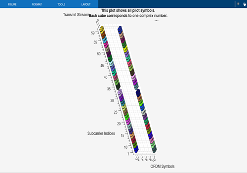
Pick pilot locations and orthogonal vectors for pilot symbols. Validate the pilot configuration and plot it.
pilotcfg.PilotLocations = {ofdmPilotGrid([1 2], 1, dataIdx(1:2:end), ...
                           [1 numOFDMSym])};
pilotcfg.PilotSymbols = cellfun(@(x) reshape(pskmod(randi([0 3], ...
              size(x,1)*size(x,3),1),4,pi/4), ...
              size(x,1),1,size(x,3)) .* ... % Random QPSK symbols
              (size(x,1)*ifft(eye(size(x,1)))), ...   % Orthogonal vectors
               pilotcfg.PilotLocations, 'UniformOutput', false);
validate(pilotcfg);
plot(pilotcfg);
Insert pilot symbols.
[pilotsym, pilotind] = pilotSignal(pilotcfg);
txGrid = zeros(pilotcfg.FFTLength - sum(pilotcfg.NumGuardBandCarriers), pilotcfg.NumSymbols, pilotcfg.NumTransmitStreams);
txGrid(pilotind) = pilotsym;
Set up the MIMO channel.
mimoChannel = comm.MIMOChannel( ...
    SampleRate=1e6, ...
    PathDelays=[0 3e-7 5e-7], ...
    AveragePathGains=[0 -2 -3], ...
    MaximumDopplerShift=20, ...
    SpatialCorrelationSpecification="None", ...
    NumTransmitAntennas=numTx, ...
    NumReceiveAntennas=numRx);
Account for the timing offset and symbol offset, remove the initial samples, and then pad with zeros to keep the signal length unchanged.
mimoChannelInfo = info(mimoChannel);
toffset = mimoChannelInfo.ChannelFilterDelay;
zeropadding = zeros(toffset,numRx);
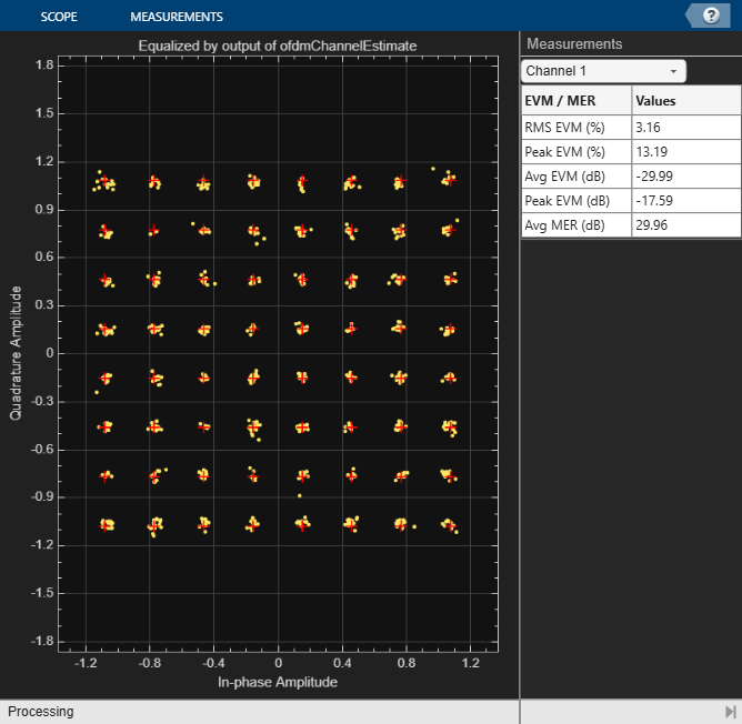
Set up the constellation diagram.
constdiag = comm.ConstellationDiagram(Title = 'Equalized by output of ofdmChannelEstimate',...
ReferenceConstellation = qammod(0:M-1,M,UnitAveragePower=true),...
EnableMeasurements = true, Position = [100 100 800 800]);
Generate random data bits and the QAM output.
for count = 1:numFrames
    dataBits = randi([0,1],[numDataSC*bps numOFDMSym-2 numStreams]);
    qamTx = qammod(dataBits,M,InputType="bit",UnitAveragePower=true);
    txGrid(dataIdx - numGuardBandCarriers1,2:end-1,:) = qamTx; % No data in the first and the last OFDM symbols
  % Perform OFDM modulation and apply beamforming.
    ofdmOut = ofdmmod(txGrid,nfft,cpLen,[1:numGuardBandCarriers1 nfft-numGuardBandCarriers2+1:nfft]');
    txOut = ofdmOut * B;
  % Pass through the MIMO channel and add noise using an AWGN channel
    channelOut = mimoChannel(txOut);
    rxIn = awgn(channelOut,SNRdB,"measured"); % add noise
  % Perform OFDM demodulation and extract the data subcarriers.
    ofdmDemodIn = [rxIn(toffset+1:end,:); zeropadding];
    rxFullGrid = ofdmdemod(ofdmDemodIn,nfft,cpLen,cpLen/2); % Use cpLen/2 for symbol sampling offset
    rxSym = rxFullGrid(dataIdx,:,:);
  % Perform channel estimation from the pilots.
    r = rxFullGrid((numGuardBandCarriers1+1:nfft-numGuardBandCarriers2),:,:);
    [hEst, nVarEst] = ofdmChannelEstimate(r, pilotcfg, cpLen);
  % Use hEst from ofdmChannelEstimate to equalize the received signal.
    dcIndx = nfft/2+1-numGuardBandCarriers1; % DC index for hEst
    hPractical = reshape(hEst([1:dcIndx-1 dcIndx+1:end],:,:,:),[],numStreams,numRx);
    eqSym = ofdmEqualize(rxSym,hPractical,nVarEst);
  % Plot a constellation diagrams of the equalized data symbols.
constdiag(reshape(eqSym(:,2:(numOFDMSym-1),:),[],1));
end
Input Arguments
Output Arguments
Algorithms
This section explains how the ofdmChannelEstimate function
computes channel estimates from pilot symbols in an OFDM waveform. The function supports
two computations, the least-squares method and the least-squares method with
denoising.
Both methods use the same core least-squares estimation procedure. The least-squares with denoising method adds structured smoothing in the frequency and time dimensions through interpolation and denoising.
To understand the least squares algorithm, consider the following OFDM system consisting of 6 transmit antennas and 8 receive antennas.
Figure-1
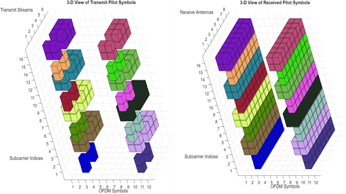
In the 3‑D MIMO-OFDM grid plots, the left plot shows the transmitted pilot symbols, and the right plot shows the corresponding received pilot symbols.
Subcarrier indices range from 1 to 16.
OFDM symbol indices range from 1 to 12.
Each color represents a pilot cluster.
The time-frequency coordinates of a cluster define its pilot locations.
In this example, the algorithm divides the MIMO‑OFDM transmit streams into two stream groups:
Stream group 1 has two transmit streams that transmit to eight receive antennas, creating a 2‑by‑8 matrix.
Stream group 2 has four transmit streams that also transmit to eight receive antennas, creating a 4‑by‑8 matrix.
The system uses six total transmit streams. Therefore, the combined least-squares estimate at any pilot location forms a 6‑by‑8 matrix by combining the two group channel estimates.
With 16 clusters, the algorithm produces 16 such matrices, one for each cluster.
Figure-2
To use the least‑squares algorithm without denoising, set the algorithm
property to 'leastsquares' in the
ofdmChannelEstimate function.
To begin channel estimation, the algorithm creates a 4‑D channel grid, h, with dimensions:
[subcarriers] × [symbols] × [transmit streams] × [receive antennas]
The algorithm initializes all entries to NaN and fills only the
positions that correspond to pilot symbol clusters.
For each pilot symbol cluster, the algorithm uses the known transmitted pilot symbols and the corresponding received measurements to form and solve a set of linear equations. Solving these equations yields a channel matrix H of size:
[number of transmit streams in the group] × [number of receive antennas]
This matrix represents the least-squares channel estimate for one cluster and is inserted into the channel grid at every pilot location belonging to that cluster.
To understand, consider the black cluster of cubes in Figure-1. The algorithm uses the transmitted pilot symbols and received measurements to solve a linear equation and compute a channel matrix H(black). The algorithm assigns this channel estimate matrix to every pilot symbol location of the black cluster.
The algorithm repeats this procedure independently for every cluster ( every color in the grid). Every cluster produces a separate least-squares channel estimate matrix, and the algorithm fills those matrices at the corresponding pilot locations in h matrix.
All remaining positions in the grid without pilot symbols remain
NaN. The pure least‑squares algorithm performs no interpolation
or smoothing beyond the pilot locations.
To use the least‑squares algorithm with denoising, set the algorithm
property to 'leastsquares-with-denoising' in the
ofdmChannelEstimate function.
The least-squares with denoising algorithm begins by performing least-squares estimation for each pilot symbol cluster. For each cluster, the algorithm computes a channel matrix H. The algorithm then computes the mean subcarrier index and the mean OFDM‑symbol index and determines the average location of each cluster.
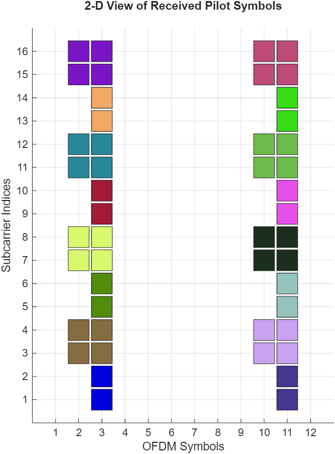
Figure-3
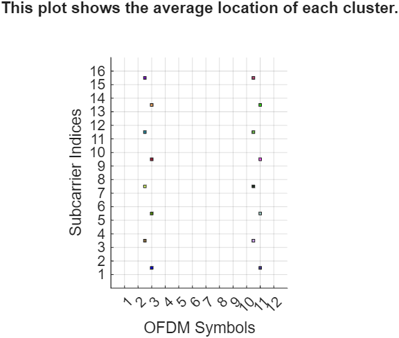
The plot shows the average location of each cluster.
The horizontal axis (OFDM Symbols) ranges from 1 to 12.
The vertical axis (Subcarrier Indices) ranges from 1 to 16.
Each colored square marks the average location of one cluster.
To prepare for frequency‑domain smoothing, the algorithm groups clusters by their average OFDM‑symbol index. All clusters whose averages fall in the same column belong to the same time slice or same symbol set.
For example, at OFDM symbol index 3, the clusters have average subcarrier positions 1.5, 5.5, 9.5, and 13.5. These clusters form the symbol‑3 set.
For the symbol-3 set, the algorithm performs the following operations:
Interpolation to fill missing subcarrier channel estimate values — For example, if the channel estimates exist at subcarriers 1.5 and 5.5, the algorithm generates estimates at 2.5, 3.5, and 4.5 by drawing a smooth curve between the two known points. It performs this interpolation for both magnitude (strength) and phase (angle) to fill missing values between subcarrier indices.
Extrapolation to lower and upper guard bands — At the edges of the frequency band, there are no pilot symbols. The algorithm extends the channel estimate values outward from the nearest pilot symbols to estimate the channel in these empty regions. It performs this extrapolation for both magnitude (strength) and phase (angle).
Spline interpolation — After the algorithm adds the extrapolated edge points, it combines all interpolated and extrapolated pilot values and applies spline interpolation to fill the missing subcarriers with a natural curve.
Denoising — After the algorithm completes interpolation and extrapolation, the channel estimate might still contain small ripples caused by noise. The denoising stage smooths these ripples while preserving the overall channel shape.
The algorithm treats the channel values across subcarriers as a wavy curve. It subtracts the mean value from the channel estimates in the symbol‑3 set and converts the result to the time domain using an inverse fast Fourier transform (IFFT) because smoothing is easier in the time domain. The algorithm then applies a soft window filter to gently reduce the ripples while keeping the main peaks intact. Next, it converts the result back to the frequency domain using a fast Fourier transform (FFT), producing a smoother curve. Finally, it adds the mean value back to the channel estimates for symbol-3 set.
The process repeats for the sets associated with symbols 2.5, 10.5, and 11.
After denoising, the algorithm removes points added outside the active subcarrier range. It then interpolates the channel estimates smoothly across OFDM symbols to fill missing time positions.
After these operations, the algorithm produces a smooth, fully populated channel estimate for every subcarrier, every OFDM symbol, every transmit stream, and every receive antenna.
Case 1 — One cluster in a symbol-set
If a symbol contains only one cluster in the symbol-set, the algorithm replicates the single cluster channel estimate across all subcarriers for that symbol. No interpolation or denoising occurs.
Case 2 — Two clusters in a symbol-set
If a symbol contains two clusters in the symbol-set, the algorithm skips guard‑band extrapolation and denoising. It uses simple linear interpolation between the two channel estimate matrices.
Extended Capabilities
Version History
Introduced in R2026a
See Also
Functions
ofdmdemod|ofdmPilotGrid|nrChannelEstimate(5G Toolbox) |lteDLChannelEstimate(LTE Toolbox) |lteULChannelEstimate(LTE Toolbox)
Objects
Blocks
- OFDM Channel Estimator (Wireless HDL Toolbox) | OFDM Demodulator Baseband