Visualize Markov Chain Structure and Evolution

This example shows how to visualize the structure and evolution of a Markov chain model using the dtmc plotting functions. Consider the four-state Markov chain that models real gross domestic product (GDP) dynamics in Create Markov Chain from Stochastic Transition Matrix.

Create the Markov chain model for real GDP. Specify the state names.

P = [0.5 0.5 0.0 0.0;
     0.5 0.0 0.5 0.0;
     0.0 0.0 0.0 1.0;
     0.0 0.0 1.0 0.0];
stateNames = ["Regime 1" "Regime 2" "Regime 3" "Regime 4"];
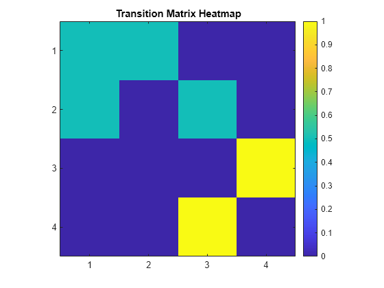
mc = dtmc(P,StateNames=stateNames);

One way to visualize the Markov chain is to plot a heatmap of the transition matrix.

figure
imagesc(P)
colorbar
axis square
h = gca;
h.XTick = 1:4;
h.YTick = 1:4;
title("Transition Matrix Heatmap")

Directed Graph

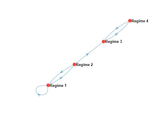
A directed graph, or digraph, shows the states in the chain as nodes, and shows feasible transitions between states as directed edges. A feasible transition is a transition whose probability of occurring is greater than zero.

Plot a default digraph of the Markov chain.

figure
graphplot(mc)

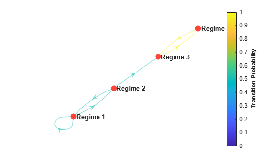
Compare probabilities of transition by specifying edge colors based on transition probability.

figure
graphplot(mc,ColorEdges=true)

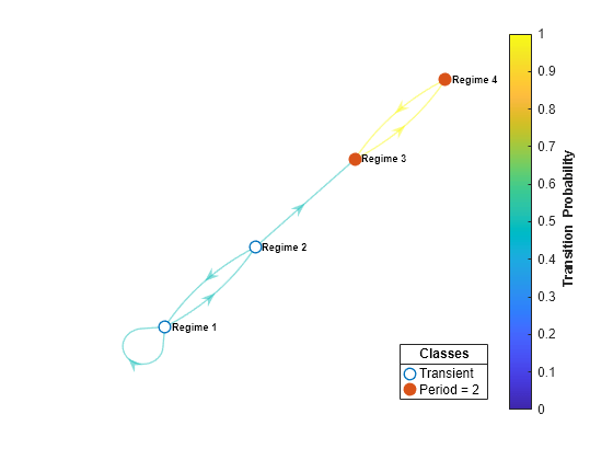
Identify recurrent and transient states by specifying node colors and markers based on state type. Return the plot handle.

figure
h = graphplot(mc,ColorEdges=true,ColorNodes=true);

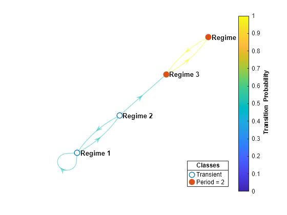
The low-mean states are transient and eventually transition to the recurrent high-mean states.

The default font size of the node labels is 8 points. Reduce the font size to 7 points.

h.NodeFontSize = 7;

Mixing Plots

The asymptotics function returns the mixing time of a Markov chain. However, but the hitprob and hittime functions enable you to visualize the mixing by plotting hitting probabilities and expected first hitting times in a digraph.

hitprob computes the probability of hitting a specified subset of target states, beginning from each state in the Markov chain. The function optionally displays a digraph of the Markov chain with node colors representing the hitting probabilities.

Plot a digraph of the Markov chain with node colors representing the probabilities of hitting regime 1.

hitprob(mc,"Regime 1",Graph=true);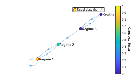

The probability of hitting regime 1 from regime 3 or 4 is 0 because regimes 3 and 4 form an absorbing subclass.

hittime computes the expected first hitting times for a specified subset of target states, beginning from each state in the Markov chain. The function optionally displays a digraph of the Markov chain with node colors representing the hitting times.

Plot a digraph of the Markov chain with node colors representing the expected first hitting times for a target subclass that contains regimes 3 and 4.

target = ["Regime 3" "Regime 4"];
hittime(mc,target,Graph=true);

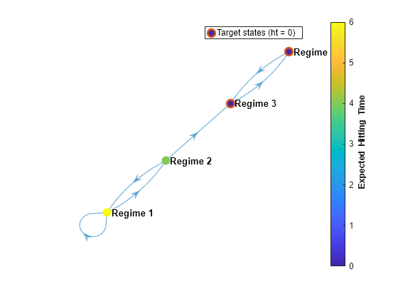
Beginning from regime 1, the expected first hitting time for the subclass is 6 time steps.

Eigenvalue Plot

An eigenvalue plot shows eigenvalues on the complex plane. eigplot returns an eigenvalue plot and identifies the:

• Perron-Frobenius eigenvalue, which is guaranteed for nonnegative matrices, using a bold asterisk.

• Spectral gap, which is the area between the radius with length equal to the second largest eigenvalue magnitude (SLEM) and the radius with a length of 1. The spectral gap determines the mixing time of the Markov chain. Large gaps indicate faster mixing, whereas thin gaps indicate slower mixing.

Plot and return the eigenvalues of the transition matrix on the complex plane.

figure
eVals = eigplot(mc)

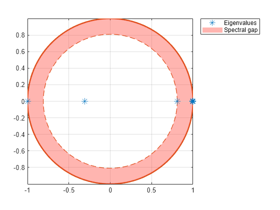
eVals = 4×1

    0.8090
   -0.3090
    1.0000
   -1.0000

Two eigenvalues have a modulus of 1, indicating that the Markov chain has a period of 2.

Redistribution Plot

A redistribution plot graphs the state redistributions $$x_t$$ from an initial distribution. Specifically, $$x_t=x_{t-1}P=x_0{P}^t$$. distplot plots redistributions using data generated by redistribute and the Markov chain object. You can plot the redistributions as a static heatmap or as animated histograms or digraphs.

Generate a 10-step redistribution from the initial distribution $$\left[\begin{array}{cccc}0.5& 0.5& 0& 0\end{array}\right]\prime$$.

numSteps = 10;
x0 = [0.5 0.5 0 0];
X = redistribute(mc,numSteps,X0=x0);

Plot the redistributions as a heatmap.

figure
distplot(mc,X)

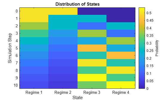
Because states 1 and 2 are transient, the Markov chain eventually concentrates the probability to states 3 and 4. Also, as the eigenvalue plot suggests, states 3 and 4 seem to have a period of 2.

Plot an animated histogram. Set the frame rate to one second.

figure
distplot(mc,X,Type="histogram",FrameRate=1);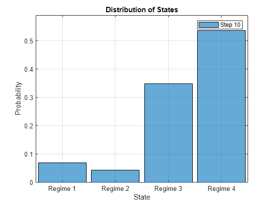

Simulation Plot

A simulation plot graphs random walks through the Markov chain starting at particular initial states. simplot plots the simulation using data generated by simulate and the Markov chain object. You can plot the simulation as a static heatmap displaying the proportion of states reached at each step, a heatmap of the realized transition matrix, or an animated digraph showing the realized transitions.

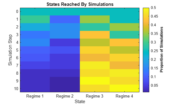
Generate 100 ten-step random walks, where each state initializes the walk 25 times.

x0 = [25 25 25 25];
X = simulate(mc,numSteps,X0=x0);

Plot the simulation as a heatmap showing the proportion of states reached at each step.

figure
simplot(mc,X);

Plot a heatmap of the realized transition matrix.

figure
simplot(mc,X,Type="transition");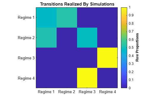

The realized transition matrix appears similar to the theoretical transition matrix.