redistribute

Compute Markov chain redistributions

Syntax

X = redistribute(mc,numSteps)

X = redistribute(mc,numSteps,'X0',x0)

Description

X = redistribute(mc,numSteps) returns data X on the evolution of a uniform distribution of states in the discrete-time Markov chain mc after it advances numSteps time steps.

X = redistribute(mc,numSteps,'X0',x0) optionally specifies the initial state distribution x0.

Examples

Visualize Evolution of State Distribution

Create a four-state Markov chain from a randomly generated transition matrix containing eight infeasible transitions.

rng('default'); % For reproducibility 
mc = mcmix(4,'Zeros',8);

mc is a dtmc object.

Plot a digraph of the Markov chain.

figure;
graphplot(mc);

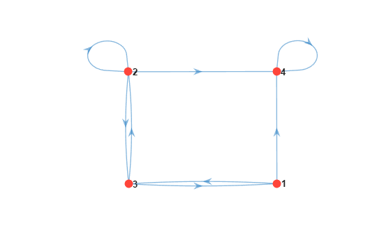
State 4 is an absorbing state.

Compute the state redistributions at each step for 10 discrete time steps. Assume an initial uniform distribution over the states.

X = redistribute(mc,10)

X = 11×4

    0.2500    0.2500    0.2500    0.2500
    0.0869    0.2577    0.3088    0.3467
    0.1073    0.2990    0.1536    0.4402
    0.0533    0.2133    0.1844    0.5489
    0.0641    0.2010    0.1092    0.6257
    0.0379    0.1473    0.1162    0.6985
    0.0404    0.1316    0.0765    0.7515
    0.0266    0.0997    0.0746    0.7991
    0.0259    0.0864    0.0526    0.8351
    0.0183    0.0670    0.0484    0.8663
    0.0168    0.0569    0.0358    0.8905
      ⋮

X is an 11-by-4 matrix. Rows correspond to time steps, and columns correspond to states.

Visualize the state redistribution.

figure;
distplot(mc,X)

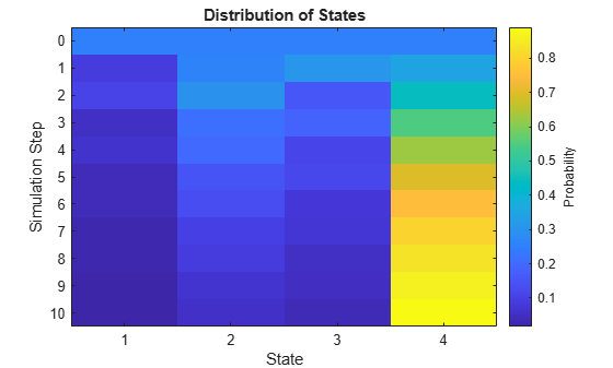
After 10 transitions, the distribution appears to settle with a majority of the probability mass in state 4.

Specify Initial Distribution for State Redistribution

Consider this theoretical, right-stochastic transition matrix of a stochastic process.

$$P=\left[\begin{array}{ccccccc}0& 0& 1/2& 1/4& 1/4& 0& 0\\ 0& 0& 1/3& 0& 2/3& 0& 0\\ 0& 0& 0& 0& 0& 1/3& 2/3\\ 0& 0& 0& 0& 0& 1/2& 1/2\\ 0& 0& 0& 0& 0& 3/4& 1/4\\ 1/2& 1/2& 0& 0& 0& 0& 0\\ 1/4& 3/4& 0& 0& 0& 0& 0\end{array}\right].$$

Create the Markov chain that is characterized by the transition matrix P.

P = [ 0   0  1/2 1/4 1/4  0   0 ;
      0   0  1/3  0  2/3  0   0 ;
      0   0   0   0   0  1/3 2/3;
      0   0   0   0   0  1/2 1/2;
      0   0   0   0   0  3/4 1/4;
     1/2 1/2  0   0   0   0   0 ;
     1/4 3/4  0   0   0   0   0 ];
mc = dtmc(P);

Plot a directed graph of the Markov chain. Indicate the probability of transition by using edge colors.

figure;
graphplot(mc,'ColorEdges',true);

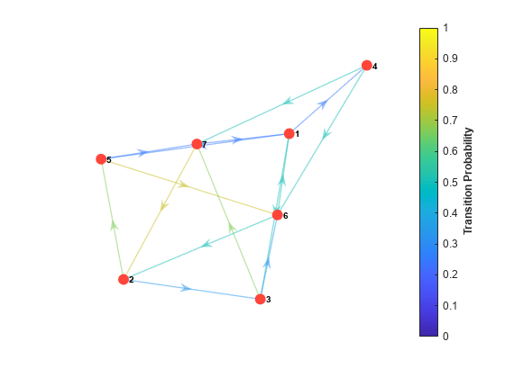
Compute a 20-step redistribution of the Markov chain using random initial values.

rng(1); % For reproducibility
x0 = rand(mc.NumStates,1);
rd = redistribute(mc,20,'X0',x0);

Plot the redistribution.

figure;
distplot(mc,rd);

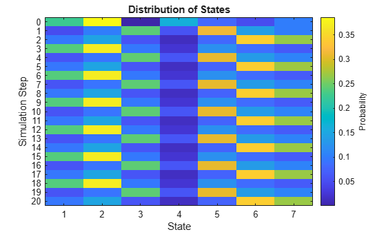
The redistribution suggests that the chain is periodic with a period of three.

Remove periodicity by creating a lazy version of the Markov chain.

lc = lazy(mc);

Compute a 20-step redistribution of the lazy chain using random initial values. Plot the redistribution.

x0 = rand(mc.NumStates,1);
lrd1 = redistribute(lc,20,'X0',x0);

figure;
distplot(lc,lrd1);

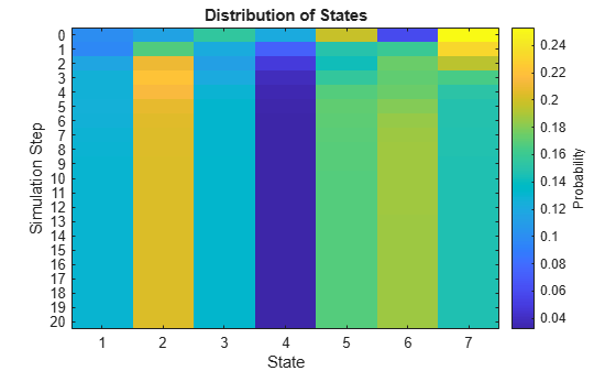
The redistribution appears to settle after several steps.

Input Arguments

mc — Discrete-time Markov chain

dtmc object

Discrete-time Markov chain with NumStates states and transition matrix P, specified as a dtmc object. P must be fully specified (no NaN entries).

numSteps — Number of discrete time steps

positive integer

Number of discrete time steps to compute, specified as a positive integer.

Data Types: double

Name-Value Arguments

Specify optional pairs of arguments as Name1=Value1,...,NameN=ValueN, where Name is the argument name and Value is the corresponding value. Name-value arguments must appear after other arguments, but the order of the pairs does not matter.

Before R2021a, use commas to separate each name and value, and enclose Name in quotes.

Example: 'X0',[0.5 0.25 0.25] specifies an initial state distribution of [0.5 0.25 0.25].

X0 — Initial distribution

nonnegative numeric vector

Initial distribution, specified as the comma-separated pair consisting of 'X0' and a nonnegative numeric vector of NumStates length. redistribute normalizes X0 so that it sums to 1.

The default is a uniform distribution of states.

Example: 'X0',[0.5 0.25 0.25]

Data Types: double

Output Arguments

X — Evolution of state probabilities

nonnegative numeric matrix

Evolution of state probabilities, returned as a (1 + numSteps)-by-NumStates nonnegative numeric matrix. The first row is X0. Subsequent rows are the redistributions at each step, which redistribute determines by the transition matrix P.

Note

If mc is ergodic, and numSteps is sufficiently large, X(end,:) approximates x = asymptotics(mc). See asymptotics.

Tips

To visualize the data created by redistribute, use distplot.

Version History

Introduced in R2017b