Pricing European Call Options Using Different Equity Models

This example illustrates how the Financial Instruments Toolbox™ is used to price European vanilla call options using different equity models.

The example compares call option prices using the Cox-Ross-Rubinstein model, the Leisen-Reimer model, and the Black-Scholes closed formula.

Define Call Instrument

Consider a European call option, with an exercise price of $30 on January 1, 2010. The option expires on Sep 1, 2010. Assume that the underlying stock provides no dividends. The stock is trading at $25 and has a volatility of 35% per annum. The annualized continuously compounded risk-free rate is 1.11% per annum.

% Option
Settle = 'Jan-01-2010';
Maturity = 'Sep-01-2010';
Strike = 30;
OptSpec = 'call';

% Stock
AssetPrice = 25;   
Sigma = .35;

Create Interest-Rate Term Structure

Use intenvset to create a RateSpec.

StartDates = '01 Jan 2010';          
EndDates =   '01 Jan 2013';
Rates = 0.0111;
ValuationDate = '01 Jan 2010';
Compounding = -1;

RateSpec = intenvset('Compounding',Compounding,'StartDates', StartDates, ...
                     'EndDates', EndDates, 'Rates', Rates,'ValuationDate', ValuationDate);

Create Stock Structure

Suppose you want to create two scenarios. The first one assumes that AssetPrice is currently $25, the option is out of the money (OTM). The second scenario assumes that the option is at the money (ATM), and therefore AssetPriceATM = 30.

AssetPriceATM = 30; 

StockSpec = stockspec(Sigma, AssetPrice);
StockSpecATM = stockspec(Sigma, AssetPriceATM);

Price Options Using Black-Scholes Closed Formula

Use the function optstockbybls to compute the price of the European call options.

% Price the option with AssetPrice = 25
PriceBLS = optstockbybls(RateSpec, StockSpec, Settle, Maturity, OptSpec, Strike);

% Price the option with AssetPrice = 30
PriceBLSATM = optstockbybls(RateSpec, StockSpecATM, Settle, Maturity, OptSpec, Strike);

Build Cox-Ross-Rubinstein Tree

Use crrtree to create a Cox-Ross-Rubinstein tree.

% Create the time specification of the tree
NumPeriods = 15;

CRRTimeSpec = crrtimespec(ValuationDate, Maturity, NumPeriods);

% Build the tree
CRRTree = crrtree(StockSpec, RateSpec, CRRTimeSpec);
CRRTreeATM = crrtree(StockSpecATM, RateSpec, CRRTimeSpec);

Build the Leisen-Reimer Tree

% Create the time specification of the tree
LRTimeSpec = lrtimespec(ValuationDate, Maturity, NumPeriods);

% Use the default method 'PP1' (Peizer-Pratt method 1 inversion)to build
% the tree
LRTree = lrtree(StockSpec, RateSpec, LRTimeSpec, Strike);
LRTreeATM = lrtree(StockSpecATM, RateSpec, LRTimeSpec, Strike);

Price Options Using the Cox-Ross-Rubinstein (CRR) Model

Use optstockbycrr to price the options using a CRR model.

PriceCRR = optstockbycrr(CRRTree, OptSpec, Strike, Settle, Maturity); 
PriceCRRATM = optstockbycrr(CRRTreeATM, OptSpec, Strike, Settle, Maturity);

Price Options Using the Leisen-Reimer (LR) Model

Use optstockbylr to price the options using a LR model.

PriceLR = optstockbylr(LRTree, OptSpec, Strike, Settle, Maturity); 
PriceLRATM = optstockbylr(LRTreeATM, OptSpec, Strike, Settle, Maturity);

Compare BLS, CRR and LR Results

sprintf('PriceBLS: \t%f\nPriceCRR: \t%f\nPriceLR:\t%f\n', PriceBLS, ...
    PriceCRR, PriceLR)

ans = 
    'PriceBLS: 	1.275075
     PriceCRR: 	1.294979
     PriceLR:	1.275838
     '

sprintf('\t== ATM ==\nPriceBLS ATM: \t%f\nPriceCRR ATM: \t%f\nPriceLR ATM:\t%f\n', PriceBLSATM, ...
    PriceCRRATM,   PriceLRATM)

ans = 
    '	== ATM ==
     PriceBLS ATM: 	3.497891
     PriceCRR ATM: 	3.553938
     PriceLR ATM:	3.498571
     '

Convergence of CRR and LR Models to a BLS Solution

The following tables compare call option prices using the CRR and LR models against the results obtained with the Black-Scholes formula.

While the CRR binomial model and the Black-Scholes model converge as the number of time steps gets large and the length of each step gets small, this convergence, except for at the money options, is anything but smooth or uniform.

The tables below show that the Leisen-Reimer model reduces the size of the error with even as few steps of 45.

Strike = 30, Asset Price = 30

-------------------------------------

#Steps LR CRR

15 3.4986 3.5539

25 3.4981 3.5314

45 3.4980 3.5165

65 3.4979 3.5108

85 3.4979 3.5077

105 3.4979 3.5058

201 3.4979 3.5020

501 3.4979 3.4996

999 3.4979 3.4987

Strike = 30, Asset Price = 25

-------------------------------------

#Steps LR CRR

15 1.2758 1.2950

25 1.2754 1.2627

45 1.2751 1.2851

65 1.2751 1.2692

85 1.2751 1.2812

105 1.2751 1.2766

201 1.2751 1.2723

501 1.2751 1.2759

999 1.2751 1.2756

Analyze the Effect of Number of Periods on Price of Options

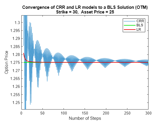
The following graphs show how convergence changes as the number of steps in the binomial calculation increases, as well as, the impact on convergence to changes to the stock price. Observe that the Leisen-Reimer model removes the oscillation and produces estimates close to the Black-Scholes model using only a small number of steps.

NPoints = 300;

% Cox-Ross-Rubinstein
NumPeriodCRR  = 5 : 1 : NPoints; 
NbStepCRR     = length(NumPeriodCRR);
PriceCRR = nan(NbStepCRR, 1);
PriceCRRATM = PriceCRR;

for i = 1 : NbStepCRR
    CRRTimeSpec = crrtimespec(ValuationDate, Maturity, NumPeriodCRR(i));
    CRRT = crrtree(StockSpec, RateSpec, CRRTimeSpec);
    PriceCRR(i) = optstockbycrr(CRRT, OptSpec, Strike,ValuationDate, Maturity) ;
    
    CRRTATM = crrtree(StockSpecATM, RateSpec, CRRTimeSpec);
    PriceCRRATM(i) = optstockbycrr(CRRTATM, OptSpec, Strike,ValuationDate, Maturity) ;
end


% Now with Leisen-Reimer
NumPeriodLR  = 5 : 2 : NPoints; 
NbStepLR     = length(NumPeriodLR);
PriceLR = nan(NbStepLR, 1);
PriceLRATM = PriceLR;

for i = 1 : NbStepLR
    LRTimeSpec = lrtimespec(ValuationDate, Maturity, NumPeriodLR(i));
    LRT = lrtree(StockSpec, RateSpec, LRTimeSpec, Strike);
    PriceLR(i) = optstockbylr(LRT, OptSpec, Strike,ValuationDate, Maturity) ;
    
    LRTATM = lrtree(StockSpecATM, RateSpec, LRTimeSpec, Strike);
    PriceLRATM(i) = optstockbylr(LRTATM, OptSpec, Strike,ValuationDate, Maturity) ;
end

First scenario: Out of the Money call option

% For Cox-Ross-Rubinstein
plot(NumPeriodCRR, PriceCRR);
hold on;
plot(NumPeriodCRR, PriceBLS*ones(NbStepCRR,1),'Color',[0 0.9 0], 'linewidth', 1.5);

% For Leisen-Reimer
plot(NumPeriodLR, PriceLR, 'Color',[0.9 0 0], 'linewidth', 1.5);

% Concentrate in the area of interest by clipping on the Y axis at 5x the
% LR Price:
YLimDelta = 5*abs(PriceLR(1) - PriceBLS);
ax = gca;
ax.YLim = [PriceBLS-YLimDelta PriceBLS+YLimDelta];

% Annotate Plot
titleString = sprintf('\nConvergence of CRR and LR Models to BLS Solution (OTM)\nStrike = %d,  Asset Price = %d', Strike , AssetPrice);
title(titleString)
ylabel('Option Price')
xlabel('Number of Steps')
legend('CRR', 'BLS', 'LR', 'Location', 'NorthEast')

Second scenario: At the Money call option

% For Cox-Ross-Rubinstein
figure;
plot(NumPeriodCRR, PriceCRRATM);
hold on;
plot(NumPeriodCRR, PriceBLSATM*ones(NbStepCRR,1),'Color',[0 0.9 0], 'linewidth', 1.5);

% For Leisen-Reimer
plot(NumPeriodLR, PriceLRATM, 'Color',[0.9 0 0], 'linewidth', 1.5);

% Concentrate in the area of interest by clipping on the Y axis at 5x the
% LR Price:
YLimDelta = 5*abs(PriceLRATM(1) - PriceBLSATM);
ax = gca;
ax.YLim = [PriceBLSATM-YLimDelta PriceBLSATM+YLimDelta];
% Annotate Plot
titleString = sprintf('\nConvergence of CRR and LR Models to BLS Solution (ATM)\nStrike = %d,  Asset Price = %d', Strike , AssetPriceATM);
title(titleString)
ylabel('Option Price')
xlabel('Number of Steps')
legend('CRR', 'BLS', 'LR', 'Location', 'NorthEast')