oe

Estimate output-error polynomial model using time-domain or frequency-domain data

Syntax

sys = oe(tt,[nb nf nk])

sys = oe(u,y,[nb nf nk])

sys = oe(data,[nb nf nk])

sys = oe(___,Name,Value)

sys = oe(tt,init_sys)

sys = oe(u,y,init_sys)

sys = oe(data,init_sys)

sys = oe(___,opt)

[sys,ic] = oe(___)

Description

Output-error (OE) models are a special configuration of polynomial models, having only two active polynomials—B and F. OE models represent conventional transfer functions that relate measured inputs to outputs while also including white noise as an additive output disturbance. You can estimate OE models using time- and frequency-domain data. The tfest command offers the same functionality as oe. For tfest, you specify the model orders using number of poles and zeros rather than polynomial degrees. For continuous-time estimation, tfest provides faster and more accurate results, and is recommended.

Estimate OE Model

sys = oe(tt,[nb nf nk]) estimates an OE model sys using the data contained in the variables of timetable tt. The software uses the first Nu variables as inputs and the next Ny variables as outputs, where Nu and Ny are determined from the dimensions of the specified polynomial orders.

sys is represented by the equation

$$y(t)=\frac{B(q)}{F(q)}u(t-nk)+e(t)$$

Here, y(t) is the output, u(t) is the input, and e(t) is the error.

The orders [nb nf nk] define the number of parameters in each component of the estimated polynomial.

To select specific input and output channels from tt, use name-value syntax to set 'InputName' and 'OutputName' to the corresponding timetable variable names.

sys = oe(u,y,[nb nf nk]) uses the time-domain input and output signals in the comma-separated matrices u,y. The software assumes that the data sample time is 1 second. To change the sample time, set Ts using name-value syntax.

sys = oe(data,[nb nf nk]) uses the time-domain or frequency-domain data in the data object data.

sys = oe(___,Name,Value) specifies model structure attributes using additional options specified by one or more name-value pair arguments. You can use this syntax with any of the previous input-argument combinations.

Configure Initial Parameters

sys = oe(tt,init_sys) uses the linear system init_sys to configure the initial parameterization of sys for estimation using the timetable tt.

sys = oe(u,y,init_sys) uses the matrix data u,y for estimation

sys = oe(data,init_sys) uses the data object data for estimation.

Specify Additional Estimation Options

sys = oe(___,opt) estimates a polynomial model using the option set opt to specify estimation behavior.

Return Estimated Initial Conditions

[sys,ic] = oe(___) returns the estimated initial conditions as an initialCondition object. Use this syntax if you plan to simulate or predict the model response using the same estimation input data and then compare the response with the same estimation output data. Incorporating the initial conditions yields a better match during the first part of the simulation.

Examples

Estimate OE Polynomial Model

Estimate an OE polynomial from time-domain data using two methods to specify input delay.

Load the estimation data.

load sdata1 tt1

Set the orders of the B and F polynomials nb and nf. Set the input delay nk to one sample. Compute the model sys.

nb = 2;
nf = 2;
nk = 1;
sys = oe(tt1,[nb nf nk]);

Compare the simulated model response with the measured output.

compare(tt1,sys)

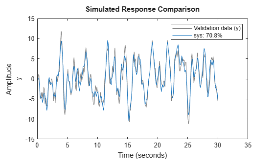
The plot shows that the fit percentage between the simulated model and the estimation data is greater than 70%.

Instead of using nk, you can also use the name-value pair argument 'InputDelay' to specify the one-sample delay.

nk = 0;
sys1 = oe(tt1,[nb nf nk],'InputDelay',1);
figure
compare(tt1,sys1)

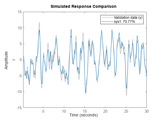
The results are identical.

You can view more information about the estimation by exploring the idpoly property sys.Report.

sys.Report

ans = 
              Status: 'Estimated using OE'
              Method: 'OE'
    InitialCondition: 'zero'
                 Fit: [1×1 struct]
          Parameters: [1×1 struct]
         OptionsUsed: [1×1 idoptions.polyest]
           RandState: [1×1 struct]
            DataUsed: [1×1 struct]
         Termination: [1×1 struct]

For example, find out more information about the termination conditions.

sys.Report.Termination

ans = struct with fields:
                 WhyStop: 'Near (local) minimum, (norm(g) < tol).'
              Iterations: 3
    FirstOrderOptimality: 0.0708
                FcnCount: 7
              UpdateNorm: 1.4809e-05
         LastImprovement: 5.1744e-06

The report includes information on the number of iterations and the reason the estimation stopped iterating.

Estimate Continuous-Time OE Model Using Frequency Response

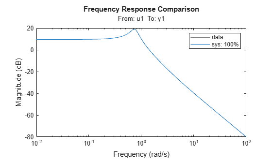
Load the estimation data.

load oe_data1 data;

The idfrd object data contains the continuous-time frequency response for the following model:

$$G(s)=\frac{s+3}{s^3+2s^2+s+1}$$

Estimate the model.

nb = 2;
nf = 3;
sys = oe(data,[nb nf]);

Evaluate the goodness of fit.

compare(data,sys);

Estimate OE Model Using Regularization

Estimate a high-order OE model from data collected by simulating a high-order system. Determine the regularization constants by trial and error and use the values for model estimation.

Load the data.

load regularizationExampleData.mat m0simdata

Estimate an unregularized OE model of order 30.

m1 = oe(m0simdata,[30 30 1]);

Obtain a regularized OE model by determining the Lambda value using trial and error.

opt = oeOptions;
opt.Regularization.Lambda = 1;
m2 = oe(m0simdata,[30 30 1],opt);

Compare the model outputs with the estimation data.

opt = compareOptions('InitialCondition','z');
compare(m0simdata,m1,m2,opt);

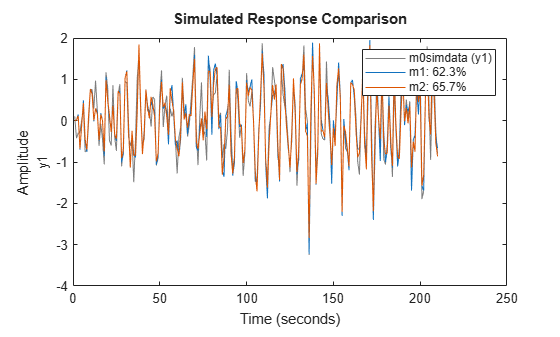
The regularized model m2 produces a better fit than the unregularized model m1.

Compare the variance in the model responses.

bp = bodeplot(m1,m2);
bp.PhaseMatchingEnabled = "on";
bp.Characteristics.ConfidenceRegion.NumberOfStandardDeviations = 3;
showConfidence(bp);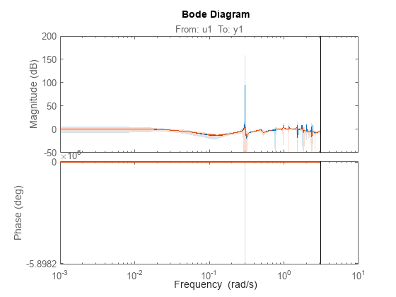

The regularized model m2 has a reduced variance compared to the unregularized model m1.

Estimate Continuous Model Using Band-Limited Discrete-Time Frequency-Domain Data

Load the estimation data data and sample time Ts.

load oe_data2.mat data Ts

An iddata object data contains the discrete-time frequency response for the following model:

$$G(s)=\frac{1000}{s+500}$$

View the estimation sample time Ts that you loaded.

Ts

Ts = 
1.0000e-03

This value matches the property data.Ts.

data.Ts

ans = 
1.0000e-03

You can estimate a continuous model from data by limiting the input and output frequency bands to the Nyquist frequency. To do so, specify the estimation prefilter option 'WeightingFilter' to define a passband from 0 to 0.5*pi/Ts rad/s. The software ignores any response values with frequencies outside of that passband.

opt = oeOptions('WeightingFilter',[0 0.5*pi/Ts]);

Set the Ts property to 0 to treat data as continuous-time data.

data.Ts = 0;

Estimate the continuous model.

nb = 1;
nf = 3;
sys = oe(data,[nb nf],opt);

Obtain Initial Conditions

Load the data, which consists of input and output data in matrix form and the sample time.

load sdata1i umat1i ymat1i Ts1i

Estimate an OE polynomial model sys and return the initial conditions in ic.

nb = 2;
nf = 2;
nk = 1;
[sys,ic] = oe(umat1i,ymat1i,[nb,nf,nk],'Ts',Ts1i);
ic

ic = 
  initialCondition with properties:

     A: [2×2 double]
    X0: [2×1 double]
     C: [0.9428 0.4824]
    Ts: 0.1000

ic is an initialCondition object that encapsulates the free response of sys, in state-space form, to the initial state vector in X0. You can incorporate ic when you simulate sys with the umat1i input signal and compare the response with the ymat1i output signal.

Input Arguments

tt — Timetable-based estimation data

timetable | cell array of timetables.

Estimation data, specified as a timetable that uses a regularly spaced time vector. tt contains variables representing input and output channels. For multiexperiment data, tt is a cell array of timetables of length Ne, where Ne is the number of experiments.

The software determines the number of input and output channels to use for estimation from the dimensions of the specified polynomial orders. The input/output channel selection depends on whether the 'InputName' and 'OutputName' name-value arguments are specified.

• If 'InputName' and 'OutputName' are not specified, then the software uses the first Nu variables of tt as inputs and the next Ny variables of tt as outputs.

• If 'InputName' and 'OutputName' are specified, then the software uses the specified variables. The number of specified input and output names must be consistent with Nu and Ny.

• For functions that can estimate a time series model, where there are no inputs, 'InputName' does not need to be specified.

For more information about working with estimation data types, see Data Domains and Data Types in System Identification Toolbox.

u, y — Matrix-based estimation data

matrices | cell array of matrices

Estimation data, specified for SISO systems as a comma-separated pair of N_s-by-1 real-valued matrices that contain uniformly sampled input and output time-domain signal values. Here, N_s is the number of samples.

For MIMO systems, specify u,y as an input/output matrix pair with the following dimensions:

• u — N_s-by-N_u, where N_u is the number of inputs.

• y — N_s-by-N_y, where N_y is the number of outputs.

For multiexperiment data, specify u,y as a pair of 1-by-N_e cell arrays, where N_e is the number of experiments. The sample times of all the experiments must match.

For time series data, which contains only outputs and no inputs, specify [],y.

Limitations

• Matrix-based data does not support estimation from frequency-domain data. You must use a data object such as an iddata object or idfrd object (see data).

For more information about working with estimation data types, see Data Domains and Data Types in System Identification Toolbox.

data — Estimation data

iddata object | frd object | idfrd object

Estimation data, specified as an iddata object, an frd object, or an idfrd object.

For time-domain estimation, data must be an iddata object containing the input and output signal values.

For frequency-domain estimation, data can be one of the following:

• Recorded frequency response data (frd (Control System Toolbox) or idfrd)

• iddata object with properties specified as follows:

  • InputData — Fourier transform of the input signal

  • OutputData — Fourier transform of the output signal

  • Domain — 'Frequency'

Time-domain estimation data must be uniformly sampled. By default, the software sets the sample time of the model to the sample time of the estimation data.

For multiexperiment data, the sample times and intersample behavior of all the experiments must match.

You can compute discrete-time models from time-domain data or discrete-time frequency-domain data. Use tfest to compute continuous-time models.

[nb nf nk] — OE model orders

integer row vector | row vector of integer matrices

OE model orders, specified as a 1-by-3 vector or a vector of integer matrices.

For a system represented by

$$y(t)=\frac{B(q)}{F(q)}u(t-nk)+e(t)$$

where y(t) is the output, u(t) is the input, and e(t) is the error, the elements of [nb nf nk] are as follows:

• nb — Order of the B(q) polynomial + 1, which is equivalent to the length of the B(q) polynomial. nb is an N_y-by-N_u matrix. N_y is the number of outputs and N_u is the number of inputs.

• nf — Order of the F polynomial. nf is an N_y-by-N_u matrix.

• nk — Input delay, expressed as the number of samples. nk is an N_y-by-N_u matrix. The delay appears as leading zeros of the B polynomial.

For estimation using continuous-time frequency-domain data, specify only [nb nf] and omit nk. For an example, see Estimate Continuous-Time OE Model Using Frequency Response.

init_sys — Linear system

idpoly model | linear model | structure

Linear system that configures the initial parameterization of sys, specified as an idpoly model, another linear model, or a structure. You obtain init_sys either by performing an estimation using measured data or by direct construction.

If init_sys is an idpoly model of the OE structure, oe uses the parameter values of init_sys as the initial guess for estimating sys. The sample time of init_sys must match the sample time of the data.

Use the Structure property of init_sys to configure initial guesses and constraints for B(q) and F(q). For example:

• To specify an initial guess for the F(q) term of init_sys, set init_sys.Structure.F.Value as the initial guess.

• To specify constraints for the B(q) term of init_sys:

  • Set init_sys.Structure.B.Minimum to the minimum B(q) coefficient values.

  • Set init_sys.Structure.B.Maximum to the maximum B(q) coefficient values.

  • Set init_sys.Structure.B.Free to indicate which B(q) coefficients are free for estimation.

If init_sys is not a polynomial model of the OE structure, the software first converts init_sys to an OE structure model. oe uses the parameters of the resulting model as the initial guess for estimating sys.

If you do not specify opt and init_sys was obtained by estimation, then the software uses estimation options from init_sys.Report.OptionsUsed.

opt — Estimation options

oeOptions option set

Estimation options, specified as an oeOptions option set. Options specified by opt include:

• Estimation objective

• Handling of initial conditions

• Numerical search method and the associated options

For examples of specifying estimation options, see Estimate Continuous Model Using Band-Limited Discrete-Time Frequency-Domain Data.

Name-Value Arguments

Specify optional pairs of arguments as Name1=Value1,...,NameN=ValueN, where Name is the argument name and Value is the corresponding value. Name-value arguments must appear after other arguments, but the order of the pairs does not matter.

Before R2021a, use commas to separate each name and value, and enclose Name in quotes.

Example: 'InputDelay',1

InputName — Input channel names

string | character vector | string array | cell array of character vectors

Input channel names, specified as a string, character vector, string array, or cell array of character vectors.

If you are using a timetable for the data source, the names in InputName must be a subset of the timetable variables.

Example: sys = oe(tt,__,'InputName',["u1" "u2"]) selects the variables u1 and u2 as the input channels from the timetable tt to use for the estimation.

OutputName — Output channel names

string | character vector | string array | cell array of character vectors

Output channel names, specified as a string, character vector, string array, or cell array of character vectors.

If you are using a timetable for the data source, the names in OutputName must be a subset of the timetable variables.

Example: sys = oe(tt,__,'OutputName',["y1" "y3"]) selects the variables y1 and y3 as the output channels from the timetable tt to use for the estimation.

Ts — Sample time

1 (default) | positive scalar

Sample time, specified as the comma-separated pair consisting of 'Ts' and the sample time in the units specified by TimeUnit. When you use matrix-based data (u,y), you must specify Ts if you require a sample time other than the assumed sample time of 1 second.

To obtain the data sample time for a timetable tt, use the timetable property tt.Properties.Timestep.

Example: oe(umat1,ymat1,___,'Ts',0.08) computes a model with sample time of 0.08 seconds.

InputDelay — Input delays

0 (default) | positive integer vector | integer scalar

Input delays for each input channel, specified as the comma-separated pair consisting of 'InputDelay' and a numeric vector.

• For continuous-time models, specify 'InputDelay' in the time units stored in the TimeUnit property.

• For discrete-time models, specify 'InputDelay' in integer multiples of the sample time Ts. For example, setting 'InputDelay' to 3 specifies a delay of three sampling periods.

For a system with N_u inputs, set InputDelay to an N_u-by-1 vector. Each entry of this vector is a numerical value that represents the input delay for the corresponding input channel.

To apply the same delay to all channels, specify 'InputDelay' as a scalar.

For an example, see Estimate OE Polynomial Model.

IODelay — Transport delays

0 (default) | scalar | numeric array

Transport delays for each input-output pair, specified as the comma-separated pair consisting of 'IODelay' and a numeric array.

• For continuous-time models, specify 'IODelay' in the time units stored in the TimeUnit property.

• For discrete-time models, specify 'IODelay' in integer multiples of the sample time Ts. For example, setting 'IODelay' to 4 specifies a transport delay of four sampling periods.

For a system with N_u inputs and N_y outputs, set 'IODelay' to an N_y-by-N_u matrix. Each entry is an integer value representing the transport delay for the corresponding input-output pair.

To apply the same delay to all channels, specify 'IODelay' as a scalar.

You can specify 'IODelay' as an alternative to the nk value. Doing so simplifies the model structure by reducing the number of leading zeros in the B polynomial. In particular, you can represent max(nk-1,0) leading zeros as input-output delays using 'IODelay' instead.

Output Arguments

sys — OE polynomial model

idpoly object

OE polynomial model that fits the estimation data, returned as an idpoly model object. This model is created using the specified model orders, delays, and estimation options. The sample time of sys matches the sample time of the estimation data. Therefore, sys is always a discrete-time model when estimated from time-domain data. For continuous-time model identification using time-domain data, use tfest.

The Report property of the model stores information about the estimation results and options used. Report has the following fields.

Report Field	Description
Status	Summary of the model status, which indicates whether the model was created by construction or obtained by estimation
Method	Estimation command used
InitialCondition	Handling of initial conditions during model estimation, returned as one of the following values: 'zero' — The initial conditions were set to zero. 'estimate' — The initial conditions were treated as independent estimation parameters. 'backcast' — The initial conditions were estimated using the best least squares fit. This field is especially useful to view how the initial conditions were handled when the InitialCondition option in the estimation option set is 'auto'.
Fit	Quantitative assessment of the estimation, returned as a structure. See Loss Function and Model Quality Metrics for more information on these quality metrics. The structure has these fields. FitPercent — Normalized root mean squared error (NRMSE) measure of how well the response of the model fits the estimation data, expressed as the percentage fitpercent = 100(1-NRMSE) LossFcn — Value of the loss function when the estimation completes MSE — Mean squared error (MSE) measure of how well the response of the model fits the estimation data FPE — Final prediction error for the model AIC — Raw Akaike Information Criteria (AIC) measure of model quality AICc — Small-sample-size corrected AIC nAIC — Normalized AIC BIC — Bayesian Information Criteria (BIC)
Parameters	Estimated values of model parameters
OptionsUsed	Option set used for estimation. If no custom options were configured, this is a set of default options. See oeOptions for more information.
RandState	State of the random number stream at the start of estimation. Empty, [], if randomization was not used during estimation. For more information, see rng.
DataUsed	Attributes of the data used for estimation, returned as a structure with the following fields. Name — Name of the data set Type — Data type Length — Number of data samples Ts — Sample time InterSample — Input intersample behavior, returned as one of the following values: 'zoh' — A zero-order hold maintains a piecewise-constant input signal between samples. 'foh' — A first-order hold maintains a piecewise-linear input signal between samples. 'bl' — Band-limited behavior specifies that the continuous-time input signal has zero power above the Nyquist frequency. InputOffset — Offset removed from time-domain input data during estimation. For nonlinear models, it is []. OutputOffset — Offset removed from time-domain output data during estimation. For nonlinear models, it is [].
Termination	Termination conditions for the iterative search used for prediction error minimization, returned as a structure with these fields. WhyStop — Reason for terminating the numerical search Iterations — Number of search iterations performed by the estimation algorithm FirstOrderOptimality — $$\infty$$-norm of the gradient search vector when the search algorithm terminates FcnCount — Number of times the objective function was called UpdateNorm — Norm of the gradient search vector in the last iteration. Omitted when the search method is 'lsqnonlin' or 'fmincon'. LastImprovement — Criterion improvement in the last iteration, expressed as a percentage. Omitted when the search method is 'lsqnonlin' or 'fmincon'. Algorithm — Algorithm used by 'lsqnonlin' or 'fmincon' search method. Omitted when other search methods are used. For estimation methods that do not require numerical search optimization, the Termination field is omitted.

For more information on using Report, see Estimation Report.

ic — Initial conditions

initialCondition object | object array of initialCondition values

Estimated initial conditions, returned as an initialCondition object or an object array of initialCondition values.

• For a single-experiment data set, ic represents, in state-space form, the free response of the transfer function model (A and C matrices) to the estimated initial states (x₀).

• For a multiple-experiment data set with N_e experiments, ic is an object array of length N_e that contains one set of initialCondition values for each experiment.

If oe returns ic values of 0 and the you know that you have non-zero initial conditions, set the 'InitialCondition' option in oeOptions to 'estimate' and pass the updated option set to oe. For example:

opt = oeOptions('InitialCondition','estimate')
[sys,ic] = oe(data,np,nz,opt)

The default 'auto' setting of 'InitialCondition' uses the 'zero' method when the initial conditions have a negligible effect on the overall estimation-error minimization process. Specifying 'estimate' ensures that the software estimates values for ic.

For more information, see initialCondition. For an example of using this argument, see Obtain Initial Conditions.

More About

Output-Error (OE) Model

The general output-error model structure is:

$$y(t)=\frac{B(q)}{F(q)}u(t-n_k)+e(t)$$

The orders of the output-error model are:

$$\begin{array}{l}nb\text{: }B(q)=b_1+b_2{q}^{-1}+\mathrm{...}+b_{nb}{q}^{-nb+1}\\ nf\text{: }F(q)=1+f_1{q}^{-1}+\mathrm{...}+f_{nf}{q}^{-nf}\end{array}$$

Continuous-Time Output-Error Model

If data is continuous-time frequency-domain data, oe estimates a continuous-time model with the following transfer function:

$$G(s)=\frac{B(s)}{F(s)}=\frac{b_{nb}{s}^{(nb-1)}+b_{nb-1}{s}^{(nb-2)}+\mathrm{...}+b_1}{s^{nf}+f_{nf}{s}^{(nf-1)}+\mathrm{...}+f_1}$$

The orders of the numerator and denominator are nb and nf, similar to the discrete-time case. However, the sample delay nk does not exist in the continuous case, and you should not specify nk when you command the estimation. Instead, express any system delay using the name-value pair argument 'IODelay' along with the system delay in the time units that are stored in the property TimeUnit. For example, suppose that your continuous system has a delay of iod seconds. Use model = oe(data,[nb nf],'IODelay',iod).

Version History

Introduced before R2006a

R2022b: Time-domain estimation data is accepted in the form of timetables and matrices

Most estimation, validation, analysis, and utility functions now accept time-domain input/output data in the form of a single timetable that contains both input and output data or a pair of matrices that contain the input and output data separately. These functions continue to accept iddata objects as a data source as well, for both time-domain and frequency-domain data.

R2018a: Advanced Options are deprecated for SearchOptions when SearchMethod is 'lsqnonlin'

Specification of lsqnonlin- related advanced options are deprecated, including the option to invoke parallel processing when estimating using the lsqnonlin search method, or solver, in Optimization Toolbox™.