Esta página se ha traducido mediante traducción automática. Haga clic aquí para ver la última versión en inglés.

append

Agregar estados al final de la ruta

Sintaxis

append(path,states)

Descripción

append(path,states) añade las muestras de estado, states, al final de path.

Ejemplos

Crear navPath basado en múltiples waypoints

Crea un objeto navPath basado en múltiples puntos de referencia en un espacio de Dubins.

dubinsSpace = stateSpaceDubins([0 25; 0 25; -pi pi])

dubinsSpace = 
  stateSpaceDubins with properties:

   SE2 Properties
                 Name: 'SE2 Dubins'
          StateBounds: [3×2 double]
    NumStateVariables: 3

   Dubins Vehicle Properties
     MinTurningRadius: 1

pathobj = navPath(dubinsSpace)

pathobj = 
  navPath with properties:

      StateSpace: [1×1 stateSpaceDubins]
          States: [0×3 double]
       NumStates: 0
    MaxNumStates: Inf

waypoints = [8 10 pi/2;
             7 14 pi/4;
             10 17 pi/2;
             10 10 -pi];
append(pathobj,waypoints)

Interpola esa ruta para que contenga exactamente 250 puntos.

interpolate(pathobj,250)

Visualice la ruta interpolada y los puntos de referencia originales.

figure
grid on
axis equal
hold on
plot(pathobj.States(:,1),pathobj.States(:,2),".b")
plot(waypoints(:,1),waypoints(:,2),"*r","MarkerSize",10)

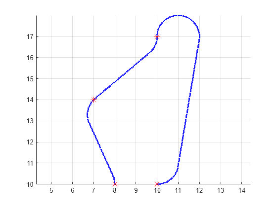
Calcular la longitud de la ruta.

len = pathLength(pathobj);
disp("Path length = " + num2str(len))

Path length = 19.4722

Crear navPath basado en múltiples puntos de referencia en el espacio de estados SE(3)

Cargue un mapa de ocupación tridimensional de una manzana de la ciudad en el espacio de trabajo. Especifique el umbral para considerar las celdas libres de obstáculos.

mapData = load("dMapCityBlock.mat");
omap = mapData.omap;
omap.FreeThreshold = 0.5;

Infle el mapa de ocupación para agregar una zona de amortiguamiento para una operación segura alrededor de los obstáculos.

inflate(omap,1)

Cree un objeto de espacio de estados SE(3) con límites para las variables de estado.

ss = stateSpaceSE3([0 220;0 220;0 100;inf inf;inf inf;inf inf;inf inf]);

Crea un objeto navPath basado en múltiples puntos de referencia en un espacio de estados SE(3).

path = navPath(ss);
waypoints = [40 180 15 0.7 0.2 0 0.1;
             55 120 20 0.6 0.2 0 0.1;
             100 100 25 0.5 0.2 0 0.1;
             130 90 30 0.4 0 0.1 0.6;
             150 33 35 0.3 0 0.1 0.6];
append(path,waypoints)

Interpola esa ruta para que contenga exactamente 250 puntos.

interpolate(path,250)

Visualice la ruta interpolada y los puntos de referencia originales.

show(omap)
axis equal
view([-10 55])
hold on
% Start state
scatter3(waypoints(1,1),waypoints(1,2),waypoints(1,3),"g","filled")
% Goal state
scatter3(waypoints(end,1),waypoints(end,2),waypoints(end,3),"r","filled")
% Intermediate waypoints
scatter3(waypoints(2:end-1,1),waypoints(2:end-1,2), ...
         waypoints(2:end-1,3),"y","filled")
% Path
plot3(path.States(:,1),path.States(:,2),path.States(:,3), ...
      "r-",LineWidth=2)

Calcular la longitud de la ruta.

len = pathLength(path);
disp("Path length = " + num2str(len))

Path length = 204.1797

Argumentos de entrada

path — objeto de ruta

objeto navPath

Objeto de ruta, especificado como un objeto navPath.

states — estados de ruta

matriz M por N de valor real

Estados de la ruta, especificados como una matriz de valores reales M por N. M es el número de estados agregados a la ruta y N es la dimensión de cada estado. La dimensión de cada estado está gobernada por el espacio de estados definido en la propiedad StateSpace de navPath. Los estados fuera del StateBounds del espacio de estados de la ruta se podan hasta los límites.

Ejemplo: [0 0 0; 1 1 0; 2 2 0]

Ejemplo: [0 0 0 1 0 0 0; 1 1 1 1 0 0 0; 2 2 1 1 0 0 0]

Tipos de datos: double

Capacidades ampliadas

Generación de código C/C++
Genere código C y C++ mediante MATLAB® Coder™.

Historial de versiones

Introducido en R2019b

Consulte también

Objetos

• navPath

Funciones

• copy | interpolate | pathLength