Measurement-Level Radar Data Generation Gallery
The radarDataGenerator provides a powerful tool for simulating statistically accurate measurement-level radar detections, enabling rapid prototyping and algorithm development for downstream tasks like tracking. While comprehensive examples of measurement-level simulations involving complex scenarios, environmental effects, and clutter modeling are available, this page provides a gallery of concise configurations and examples that you can easily incorporate into your own designs. Each example below highlights a specific feature or configuration of the radarDataGenerator and can be run independently. Some of the examples use radarDataGenerator as a sensor within a radarScenario to leverage built-in trajectory and target management features.
Configuring Radar Detection Capability
Create a radarDataGenerator that can detect a target with a radar cross section (RCS) of 2 dBsm, 80% of the time at 10 km and a probability of false alarm of 1e-5.
clear
radar = radarDataGenerator(1, 'No scanning', ...
    'ReferenceRCS',2,...
    'ReferenceRange',10e3,...
    'DetectionProbability',0.80,...
    'FalseAlarmRate',1e-5);
radarDataGenerator is a statistical model that lets you specify a set of detection-related parameters to generate detections, rather than starting from a desired SNR as is typical in power-level design analysis. The radar's detection capability is related to the DetectionProbability (probability of detection), ReferenceRange (reference range for a given probability of detection), ReferenceRCS (reference radar cross section for a given probability of detection), and FalseAlarmRate (false alarm rate) and is encapsulated by the RadarLoopGain (radar system gain) property. The RadarLoopGain is an internally-generated, read-only property that encapsulates all the radar internal parameters related to detection, such as transmit power, antenna gain, and noise figure, into a single value. RadarLoopGain is computed using the formula
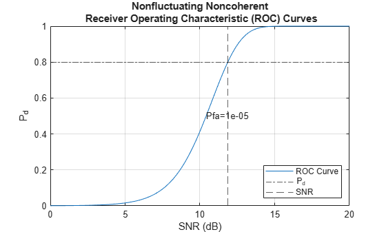
where is the ReferenceRange, is the ReferenceRCS, and is the signal-to-noise ratio required for the specified DetectionProbability and FalseAlarmRate. To better understand how the RadarLoopGain is computed, first, plot the ROC curve using the false alarm rate set above. Then, compute the SNR for a probability of detection of 0.80.
[Pd,SNR] = rocpfa(radar.FalseAlarmRate,SignalType="NonfluctuatingNoncoherent");
figure;
rocpfa(radar.FalseAlarmRate,SignalType="NonfluctuatingNoncoherent"); % create plot
hold on;
yline(radar.DetectionProbability,'-.')
idx = Pd < 1; % because multiple SNR values have Pd of 1
refSNR = rocinterp(Pd(idx),SNR(idx),radar.DetectionProbability,'pd-snr');
xline(refSNR,'--')
legend({'ROC Curve','P_d','SNR'},'Location','southeast')
Lastly, compute the RadarLoopGain using the formula and then compare it with the value stored inside the radarDataGenerator.
pow2db(db2pow(refSNR) * radar.ReferenceRange^4/db2pow(radar.ReferenceRCS))
ans =
169.8635
radar.RadarLoopGain
ans =
169.8768
After the radar is set up, you can place a target anywhere. Place a target with an RCS of 10 dBsm 100 meters away from the radar platform along the x-direction.
tgt1 = struct(...
    'PlatformID',1, ...
    'Position', [100 0 0], ...
    'Velocity', [0 0 0],...
    'Signatures',{{rcsSignature('Pattern',10)}});
Compute the predicted SNR using the formula above.
predictedSNR = radar.RadarLoopGain + tgt1.Signatures{1}.Pattern(1) - 4*pow2db((norm(tgt1.Position)))predictedSNR = 99.8768
Detect the target at time 0.
det = radar(tgt1,0);
det = det{1};
Compare the measured SNR with the predicted SNR. det is an objectDetection object of detections that contains an ObjectAttributes struct. The SNR is a field in that structure.
measSNR = det.ObjectAttributes{1}.SNRmeasSNR = 99.8768
Configuring a radarDataGenerator from a Power-Level Design
If you want to incorporate many design parameters into your radar such as transmit power, number of pulses per dwell, antenna characteristics, etc., then you can export a radarDataGenerator directly from the radarDesigner App. See Radar Design Part I: From Power Budget Analysis to Dynamic Scenario Simulation to learn how.
Understanding Resolution
Range
Range resolution refers to a radar system's ability to distinguish between two closely spaced targets along the range dimension. When targets are too close together to be individually resolved, they appear as a single merged detection. To determine if two detections are to be separated or merged in the range dimension, first compute the following for each detection.
Then, if two detections are in the same range bin, they are merged. Otherwise, they are treated as separate detections. It is important to note that the ranges reported in the detections are not rounded. The rounding above is only used to determine if detections should be merged.
This methodology can lead to interesting edge effects. Below, we show a few illustrative examples on resolving and merging target detections. To show the range resolution, first create a staring radar with no false alarms or noise with a probability of detection equal to 1. Also set the range resolution to 2 meters for simplicity. Targets separated by at least 2 meters will be resolved. As we'll see below, some targets separated by less than 2 meters will also be resolved due to round off effects.
clear
radar = radarDataGenerator(1,"No scanning",...
    'RangeResolution',2, ...
    'DetectionProbability',1,...
    'HasFalseAlarms',false,...
    'TargetReportFormat','Detections', ...
    'HasNoise',false,...
    'DetectionCoordinates','Sensor rectangular');
Create two target structs as placeholders. Set their positions later for each example.
tgt1 = struct(...
    'PlatformID',1, ...
    'Position', [0 0 0], ...
    'Signatures',{{rcsSignature('Pattern',10)}});

tgt2 = struct(...
    'PlatformID',2, ...
    'Position', [0 0 0], ...
    'Signatures',{{rcsSignature('Pattern',10)}});
Then plot the ground truth positions and the detection coordinates. Delineate the range bin boundaries using dashed lines.
tgt1.Position(1) = 97; % m
tgt2.Position(1) = 99; % m
helperPlotRangeRes(radar,tgt1,tgt2)
title("Resolved Targets Separated by 2 Meters")
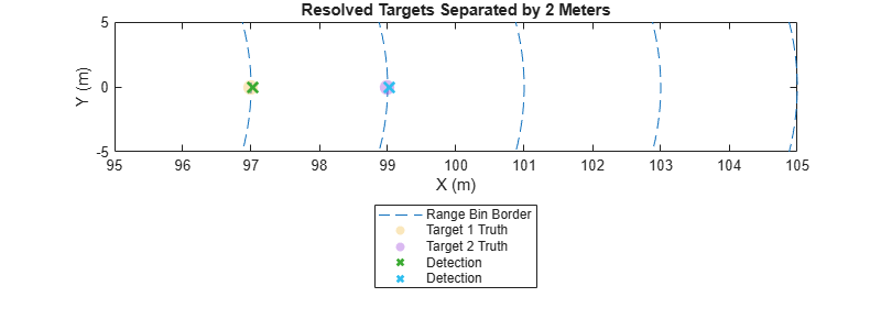
In the first example, the targets are separated by 2 meters and are each located in separate range bins. As a result, the targets are reported as separate detections.
tgt1.Position(1) = 97; % m
tgt2.Position(1) = 98.9; % m
helperPlotRangeRes(radar,tgt1,tgt2)
title("Merged Targets Separated by 1.9 Meters")
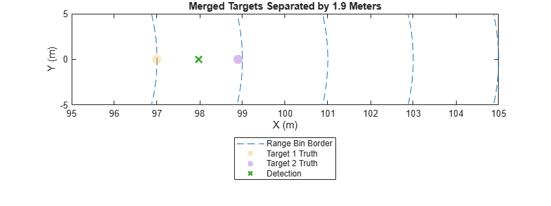
In the second example, the targets are not resolvable because both targets are located within the same range bin.
tgt1.Position(1) = 98; % m
tgt2.Position(1) = 99.1; % m
helperPlotRangeRes(radar,tgt1,tgt2)
title("Edge Case:  Resolved Targets Separated by 1.1 Meters")
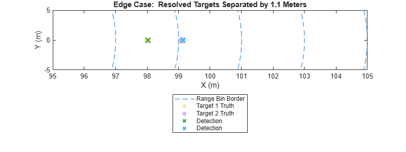
In the third example, the targets are resolvable because the targets are each located in different range bins. Two separate detections are reported despite the fact that the targets are only 1.1 meters apart, which is less than the range resolution of 2 meters.
Also notice that although there is no noise in these examples, the detections are slightly biased to be farther than the ground truth position. This is caused by refraction, which is discussed in the section below.
function helperCircle(rs)
    color = colororder;
    for r = rs
        ang=linspace(-.3,.3,100);
        xp=r*cos(ang);
        yp=r*sin(ang);
        plot(xp,yp,'--','Color',color(1,:),'DisplayName','Range Bin Border');
        hold on;
    end
end

function helperPlotRangeRes(radar,tgt1,tgt2)
    f = figure;
    f.Position(3:4) = [800 300];
    helperCircle(radar.RangeResolution*((45:53)-.5))
    lg = legend('Location','southoutside');
    lg.String = lg.String(1);
    scatter(tgt1.Position(1),tgt1.Position(2),100,'filled','MarkerFaceAlpha',.3,'DisplayName','Target 1 Truth')
    scatter(tgt2.Position(1),tgt2.Position(2),100,'filled','MarkerFaceAlpha',.3,'DisplayName','Target 2 Truth')

    xlim([95,105])
    ylim([-5 5])
    xticks(95:105)
    xlabel('X (m)')
    ylabel('Y (m)')

    dets =radar([tgt1,tgt2],0);
    cellfun(@(s) scatter(s.Measurement(1),s.Measurement(2),100,'x','LineWidth',2,'DisplayName','Detection'), dets,'UniformOutput',false);
end
Azimuth
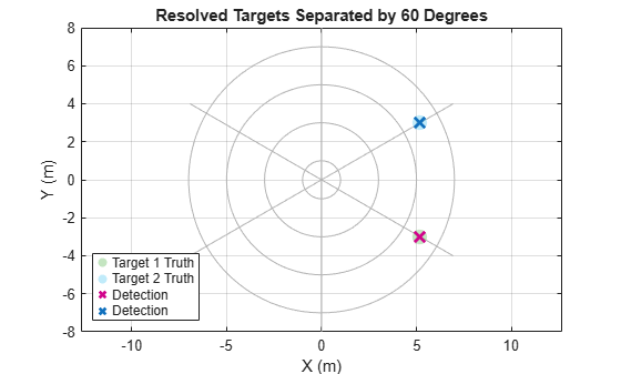
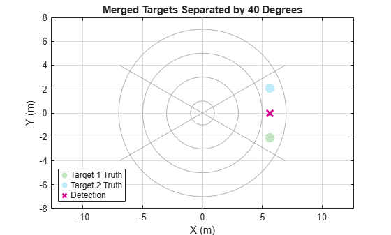
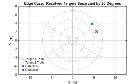
The same logic applies to resolving targets in azimuth and elevation. Set the azimuth resolution to 60 degrees and plot the target locations and the corresponding detections.
release(radar);
radar.AzimuthResolution = 60;
radar.FieldOfView = 180;

% Angles to test
a1 = [-30 -20 20];
a2 = [30 20 40];
titles = {"Resolved Targets Separated by 60 Degrees",...
    "Merged Targets Separated by 40 Degrees",...
    "Edge Case:  Resolved Targets Separated by 20 Degrees"};

for ii = 1:numel(a1)
    [x,y] = pol2cart(deg2rad(a1(ii)),6);
    tgt1.Position(1:2) = [x y];
    [x,y] = pol2cart(deg2rad(a2(ii)),6);
    tgt2.Position(1:2) = [x y];

    helperCreatePPI(radar)
    scatter(tgt1.Position(1),tgt1.Position(2),100,'filled','MarkerFaceAlpha',.3,'DisplayName','Target 1 Truth')
    scatter(tgt2.Position(1),tgt2.Position(2),100,'filled','MarkerFaceAlpha',.3,'DisplayName','Target 2 Truth')
    dets =radar([tgt1,tgt2],0);
    detPos = cellfun(@(s) scatter(s.Measurement(1),s.Measurement(2),100,'x','LineWidth',2,'DisplayName','Detection'), dets,'UniformOutput',false);

    legend('Location','southwest')
    grid on
    title(titles{ii})
    xlabel('X (m)')
    ylabel('Y (m)')
end
function helperCreatePPI(radar)
    figure;
    maxRange = 8;
    % Range rings
    rangeRings = (0:radar.RangeResolution:(maxRange-radar.RangeResolution)) + .5*radar.RangeResolution;
    for r = rangeRings
        theta = linspace(0, 2*pi, 100);
        plot(r*cos(theta), r*sin(theta),'Color',[.7 .7 .7], 'LineWidth', 0.5, 'HandleVisibility', 'off');
        hold on
    end

    % Azimuth marks
    azimuths = (0:radar.AzimuthResolution:360) + .5*radar.AzimuthResolution;
    for az = azimuths
        xline = maxRange * cos(deg2rad(az));
        yline = maxRange * sin(deg2rad(az));
        plot([0 xline], [0 yline],'Color',[.7 .7 .7], 'LineWidth', 0.3, 'HandleVisibility', 'off');
    end
    axis equal

end
Range Rate
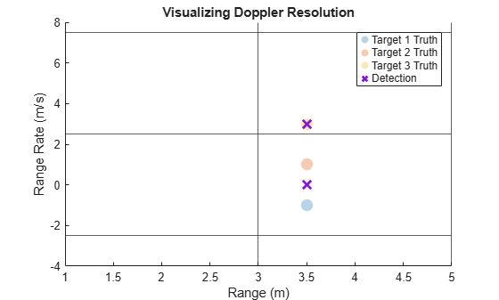
One advantage of radar is that targets can also be resolved using Doppler velocity or range rate and not just their locations. To see this, create three targets with the same position and different velocities. Set the target velocities such that two targets are in the same Doppler bin and the third is not.
% Target 1 and 2 will be merged
tgt1 = struct(...
    'PlatformID',1, ...
    'Position', [3.5 0 0], ...
    'Velocity', [-1 0 0]);

tgt2 = struct(...
    'PlatformID',2, ...
    'Position', [3.5 0 0], ...
    'Velocity', [1 0 0]);

% Target 3 is in a separate Doppler bin
tgt3 = struct(...
    'PlatformID',3, ...
    'Position', [3.5 0 0], ...
    'Velocity', [3 0 0]);

release(radar);
radar.HasRangeRate = true;
radar.RangeRateResolution = 5;

dets = radar([tgt1,tgt2,tgt3],0);
detRange = cellfun(@(s) s.Measurement(1), dets);
detRangeRate = cellfun(@(s) s.Measurement(4), dets);

figure;
scatter(tgt1.Position(1),tgt1.Velocity(1),100,'filled','MarkerFaceAlpha',.3,'DisplayName','Target 1 Truth')
hold on
scatter(tgt2.Position(1),tgt2.Velocity(1),100,'filled','MarkerFaceAlpha',.3,'DisplayName','Target 2 Truth')
scatter(tgt3.Position(1),tgt3.Velocity(1),100,'filled','MarkerFaceAlpha',.3,'DisplayName','Target 3 Truth')
scatter(detRange,detRangeRate,100,'x','LineWidth',2,'DisplayName','Detection')
xline(radar.RangeResolution * ((0:2)+.5),'HandleVisibility', 'off')
yline(radar.RangeRateResolution * ((-1:1)+.5),'HandleVisibility', 'off')
xlabel('Range (m)')
ylabel('Range Rate (m/s)')
title('Visualizing Doppler Resolution')
legend
Measurement Ambiguity
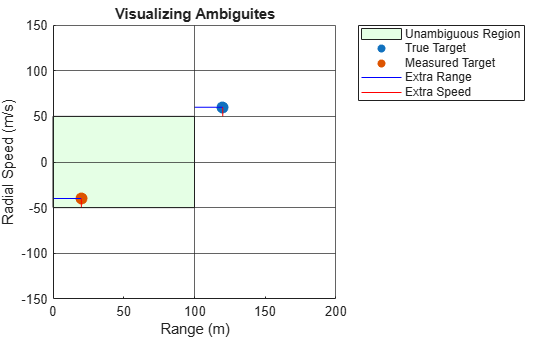
In real radar systems, ambiguities in range and Doppler measurements arise due to transmitted waveforms being periodic. Specifically, the range ambiguity stems from scenarios in which targets are far enough that their reflected return arrives back at the receiver only after the next pulse has already been transmitted. The ambiguity lies in determining which transmission the received signal originated from. Doppler ambiguity is a result of the Nyquist limit defined by half the pulse repetition frequency (PRF). For cases when a target is moving with a Doppler shift higher than half the PRF, the Doppler will be aliased.
To observe the effects of ambiguity, set the maximum unambiguous range to 100 meters and the maximum unambiguous radial speed to 50 m/s. Then, create a moving target at a range of 120 meters and a radial speed of 60 m/s.
clear maxRange = 100; maxSpeed = 50; radar = radarDataGenerator(1,"No scanning",... 'HasRangeRate',true,... 'RangeResolution',2, ... 'DetectionProbability',1,... 'HasFalseAlarms',false,... 'TargetReportFormat','Detections', ... 'HasNoise',false,... 'DetectionCoordinates','Sensor rectangular', ... 'HasRangeAmbiguities',true,... 'MaxUnambiguousRange',maxRange,... 'HasRangeRateAmbiguities',true,... 'MaxUnambiguousRadialSpeed',maxSpeed); trueRange =120; trueSpeed =
60; tgt1 = struct(... 'PlatformID',1, ... 'Position', [trueRange 0 0], ... 'Velocity', [trueSpeed 0 0]); % Run the radar det =radar(tgt1,0); meas = det{1}.Measurement; extraRange = trueRange - maxRange; extraSpeed = trueSpeed - maxSpeed; figure; x =radar.MaxUnambiguousRange * [0 1 1 0]; y =radar.MaxUnambiguousRadialSpeed * [-1 -1 1 1]; patch(x,y,'green','FaceAlpha',.1,'DisplayName','Unambiguous Region') hold on xline(radar.MaxUnambiguousRange * (0:2),'HandleVisibility', 'off') yline(radar.MaxUnambiguousRadialSpeed * (-3:3),'HandleVisibility', 'off') scatter(tgt1.Position(1),tgt1.Velocity(1),80,'o','filled','DisplayName','True Target') scatter(meas(1),meas(4),80,'o','filled','DisplayName','Measured Target') if trueRange > maxRange plot([maxRange trueRange],[trueSpeed,trueSpeed],'b','DisplayName','Extra Range') plot([0 meas(1)],[meas(4),meas(4)],'b','HandleVisibility','off') end if abs(trueSpeed) > maxSpeed plot([meas(1) meas(1)],[-sign(trueSpeed) * maxSpeed,meas(4)],'red','DisplayName','Extra Speed') plot([trueRange trueRange],[sign(trueSpeed) * maxSpeed,trueSpeed],'red','HandleVisibility','off') end legend('Location','bestoutside') xlabel('Range (m)') ylabel('Radial Speed (m/s)') title('Visualizing Ambiguites')
Detecting Extended Targets
In some design cases, modeling targets as point targets may not be sufficient. You can create extended targets by setting the Dimensions property of the target struct. The Dimensions property defines the following:
Length (x-axis)
Width (y-axis)
Height (z-axis)
Origin Offset (three element vector specifying the offsets in the x, y, and z axes respectively)
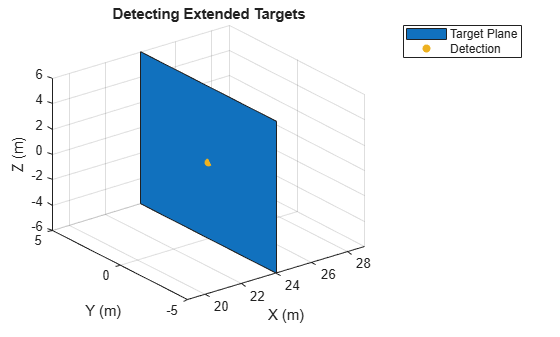
To visualize how the radarDataGenerator handles extended targets, first define an extended target in front of the radar. Set the dimensions of the target such that it approximates a panel that faces the radar. Change the x-value of the origin offset to see the plane closest to the radar move in the plot below.
clear
tgt1 = struct(...
    'PlatformID',1, ...
    'Position', [20 0 0], ...
    'Velocity', [0 0 0],...
    'Dimensions',struct('Height',12,'Width',10,'Length',1e-3,...
    'OriginOffset',[-4 0 0]));
The expected range of the detections on the surface of the target that is closest to the radar is:
expectedRange = tgt1.Position(1) - tgt1.Dimensions.Length/2 - tgt1.Dimensions.OriginOffset(1)
expectedRange =
23.9995
Then, create a staring radarDataGenerator configured with no noise or false alarms. Make sure the detection probability is set to 1 and the field of view is set large enough to include the whole target. Lastly, set the azimuth and elevation resolutions high enough such that the cross-range resolution is finer than the cross-range extent of the target. The cross-range resolution is approximately where is the angular resolution in radians.
radar = radarDataGenerator(1,"No scanning",...
    'HasElevation',true,...
    'HasFalseAlarms',false,...
    'TargetReportFormat','Detections', ...
    'AzimuthResolution',3,...
    'ElevationResolution',5,...
    'DetectionProbability',1,...
    'HasNoise',false,...
    'FieldOfView',[180,180],...
    'DetectionCoordinates','Sensor rectangular');
Detect the target and plot the detections and the target surface closest to the radar.
dets =radar(tgt1,0); % get detections

colors = colororder;
figure;
x = expectedRange * ones(1,4);
y = tgt1.Dimensions.Width/2 * [-1 -1 1 1];
z = tgt1.Dimensions.Height/2 * [1 -1 -1 1];
fill3(x,y,z,colors(1,:),'DisplayName','Target Plane')
hold on;

for detIdx = 1:numel(dets)
    meas = dets{detIdx}.Measurement;
    scatter3(meas(1),meas(2),meas(3),35,colors(3,:),"filled",'DisplayName','Detection');
end

xlabel('X (m)')
ylabel('Y (m)')
zlabel('Z (m)')
title('Detecting Extended Targets')
grid
grid minor
xlim(expectedRange + [-5 5])
lg = legend;
lg.String = lg.String(1:2);

The radarDataGenerator also allows you to cluster the detections from the same target. To do this, release the radar and set the TargetReportFormat to Clustered detections.
release(radar)
radar.TargetReportFormat = "Clustered detections";
dets =radar(tgt1,0);

figure; % Plot the detections
x = expectedRange * ones(1,4);
y = tgt1.Dimensions.Width/2 * [-1 -1 1 1];
z = tgt1.Dimensions.Height/2 * [1 -1 -1 1];
fill3(x,y,z,colors(1,:),'DisplayName','Target Plane')
hold on;

for detIdx = 1:numel(dets)
    meas = dets{detIdx}.Measurement;
    scatter3(meas(1),meas(2),meas(3),35,colors(3,:),"filled",'DisplayName','Detection');
end

xlabel('X (m)')
ylabel('Y (m)')
zlabel('Z (m)')
title('Detecting Extended Targets')
xlim(expectedRange + [-5 5])
grid
lg = legend;
lg.String = lg.String(1:2);
Detection Coordinates
For convenience, the radarDataGenerator allows you to report detections in four different coordinate systems specified in Radar Coordinate Systems and Frames. Choosing the right coordinate system in the radar itself can save you from having to change coordinate systems manually. To understand each coordinate system, first create a radarScenario and place a target at 100 meters in the x-direction and 33 meters in the y-direction.
clear
% Create radar scenario
scene = radarScenario('UpdateRate',0);

% Add target
targetPlat = platform(scene,'Position',[100 33 0], ...
    'Signatures',{rcsSignature('Pattern',ones(2,2)*10)});
Sensor Rectangular
Set the detection coordinates to Sensor rectangular to report the target locations in rectangular coordinates relative to the radar sensor. To see this, create a radar with a wide field of view and a detection probability of 1. Set the MountingLocation and the MountingAngles of the sensor to [25 0 0] and [0 0 0], respectively.
mountingLocation = [25 0 0];
mountingAngles = [0 0 0];
radar = radarDataGenerator(1, 'No scanning', ...
    'UpdateRate', 1, ...
    'DetectionProbability',1,...
    'FieldOfView',[180 180],...,
    'HasNoise', false,...
    'MountingLocation',mountingLocation,...
    'MountingAngles', mountingAngles,...
    'DetectionCoordinates','Sensor rectangular');
Then, place the radar on a platform in the scenario.
% Place radar sensor on a stationary platform
radarBodyPos = [50,0,0]; % East-North-Up Cartesian Coordinates
radarBodyOrientation = [0 0 0];  % (deg) Yaw, Pitch, Roll
radarPlat = platform(scene,'Position',radarBodyPos,'Sensors',radar,'Orientation',radarBodyOrientation);
In this case, the mounting angles and radar body orientation are zero and can subsequently be ignored. As a result, the expected position measured by the radar is the following:
predictedSensorMeasurement = targetPlat.Position - radarBodyPos - mountingLocation
predictedSensorMeasurement = 1×3

    25    33     0
Detect the target in the scene and display the measured target position.
det = detect(scene);
det{1}.Measurement
ans = 3×1
25.0000
33.0000
0
Sensor Spherical
You can change the reported coordinates so that they are in spherical coordinates with all else being the same as the example above. To see this, change the radar's detection coordinates to Sensor spherical and detect the target.
release(radar)
radar.DetectionCoordinates = 'Sensor spherical';

restart(scene)
det = detect(scene);
det{1}.Measurement
ans = 2×1
52.8533
41.4005
Check that the measured azimuth is the same as that measured in rectangular coordinates.
rad2deg(atan(predictedSensorMeasurement(2)/predictedSensorMeasurement(1)))
ans =
52.8533
Check that the measured range is the same as that measured in rectangular coordinates.
norm(predictedSensorMeasurement)
ans =
41.4005
Body
When the detection coordinates are set to Body, the target is reported in coordinates relative to the scenario platform's body. As a result, the mounting location set in the radarDataGenerator will not be included in the measured target location. To observe this, set the detection coordinates to Body and detect the target. Note that the detection coordinates are reported in rectangular coordinates in this mode.
release(radar)
radar.DetectionCoordinates = 'Body';

restart(scene)
det = detect(scene);
det{1}.Measurement
ans = 3×1
50.0000
33.0000
0
Check that the measured target location is only a function of the target and radar platform locations.
predictedBodyMeasurement = targetPlat.Position - radarBodyPos
predictedBodyMeasurement = 1×3

    50    33     0
Scenario
In many applications, it is more convenient to report target locations in the scenario coordinates or world coordinates. For example, if your scenario has multiple sensors, it might be convenient to use a single reference coordinate system between all the sensors. In order to report detections in the scenario coordinate system, you must first measure the position and orientation of the sensor itself. In the radarScenario, this is done for you.
To report detections in the scenario frame, first set the radar's detection coordinates to Scenario. Then, detect the target and display its location.
release(radar)
radar.DetectionCoordinates = 'Scenario';

% IMPORTANT: Allows the radarDataGenerator to use the RCS of the target platform
radar.Profiles = platformProfiles(scene);

det = detect(scene);
det{1}.Measurement
ans = 3×1

  100.0000
   33.0000
         0
To see what information about the radar platform the radarScenario uses in its calculations, run the following command:
pose(radarPlat)
ans = struct with fields:
        Orientation: [1×1 quaternion]
           Position: [50 0 0]
           Velocity: [0 0 0]
       Acceleration: [0 0 0]
    AngularVelocity: [0 0 0]
Simulating a Tracking Radar
In addition to outputting detections, the radarDataGenerator can also simulate measurements that have already gone through the data association step that assigns detections to targets. In this mode, the output is of an objectTrack object. Just as you can change properties of the radar like the range resolution, you can also change the following tracking-related properties of the radarDataGenerator:
The tracker model: You can choose from a variety of Kalman filter models (alpha-beta, linear, extended, and unscented) and state dimensions (constant velocity, acceleration, or turn rate) by setting the
FilterInitializationFcn. You can also define your own model.Confirmation Threshold: You can set how many and how often detections must occur in order to start a new track by specifying the
ConfirmationThresholdproperty.Deletion Threshold: You can set how many missed detections and how often they must occur in order to delete a track by specifying the
DeletionThresholdproperty.Coordinate System: You can choose to report tracks in the scenario, body, or sensor frames by specifying the
TrackCoordinatesproperty.
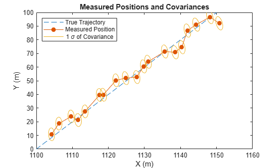
To explore the tracking functionality, create a simple tracking radar that uses a constant-velocity unscented Kalman filter. Make the confirmation threshold 3 detections for every 4 dwells and the deletion threshold 2 misses in 3 dwells. Use a radarScenario so that you can easily create and retrieve information from platform trajectories. Report the tracks in scenario coordinates. Also, set the range and azimuth biases to 0.15 so that the covariance ellipses are more visible. Lastly, Make sure HasINS is set to true. INS stands for inertial navigation system and allows you to pass in the radar's pose so that the detections can be reported in scenario coordinates.
clear
% Noise is on by default
radar = radarDataGenerator(1,"No scanning",...
    "HasFalseAlarms",false,...
    "AzimuthBiasFraction",.05,...
    "AzimuthResolution",5,...
    'RangeBiasFraction',.1,...
    'RangeResolution',10,...
    'FieldOfView',[180,180],...
    'RangeLimits',[1,1e9],...
    'UpdateRate',.2,...
    'HasElevation',true,...
    'HasINS',true,... % necessary to report in scenario coordinates
    'TargetReportFormat','Tracks',...
    'FilterInitializationFcn',@initcvukf,...
    'ConfirmationThreshold',[3 4],...
    'DeletionThreshold',[2 3]);

% Create radar scenario
scene = radarScenario('UpdateRate',0);

% Place radar on a stationary platform
radarPos = [0,0,0]; % East-North-Up Cartesian Coordinates
radarOrientation = [0 0 0];  % (deg) Yaw, Pitch, Roll
radarPlat = platform(scene,'Position',radarPos,'Sensors',radar,'Orientation',radarOrientation);

% Create target with specified trajectory
waypoints = [1.1e3 0 0; 1.15e3 1e2 0];
trajectory = waypointTrajectory('TimeOfArrival',[0; 1e2],'Waypoints',waypoints);
targetPlat = platform(scene,'Trajectory',trajectory, ...
    'Signatures',{rcsSignature('Pattern',ones(2,2)*10)});

% IMPORTANT: Allows the radarDataGenerator to use the RCS of the target platform
radar.Profiles = platformProfiles(scene);

rng('default')
allTracks = [];
while scene.advance
    tgtPoses = targetPoses(radarPlat);
    ins = pose(radarPlat);
    tracks =radar(tgtPoses,ins,scene.SimulationTime);

    % Append any new track data
    allTracks = [allTracks;tracks];
end
targetLocations = arrayfun(@(x) [x.State(1),x.State(3)] ,allTracks ,'UniformOutput' ,false);
targetLocations = cell2mat(targetLocations);

figure;
colors = colororder;
plot(waypoints(:,1),waypoints(:,2),'--','DisplayName','True Trajectory')
hold on
plot(targetLocations(:,1),targetLocations(:,2),'.-','MarkerSize',20,'Color',colors(2,:),'DisplayName','Measured Position')
lg = legend('Location','northwest');
lg.String = lg.String(1:2);
arrayfun(@(x) helperPlotCov(x,colors(3,:)),allTracks)
lg.String = lg.String(1:3);
ylim([0 waypoints(2,2)])
xlabel('X (m)')
ylabel('Y (m)')
title('Measured Positions and Covariances')
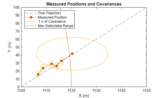
Track Deletion
To observe the deletion of a track, set the radar's upper range limit to a value less than the maximum range of the target trajectory. Notice that after the first missed detection, the covariance ellipse grows. Then, after the second missed detection and its subsequent deletion, the target and its ellipse are not plotted at all.
release(radar);
radar.RangeLimits = [1 1120];

% Create radar scenario
scene = radarScenario('UpdateRate',0);

% Place radar on a stationary platform
radarPlat = platform(scene,'Position',radarPos,'Sensors',radar,'Orientation',radarOrientation);

% Create target with specified trajectory
trajectory = waypointTrajectory('TimeOfArrival',[0; 1e2],'Waypoints',waypoints);
targetPlat = platform(scene,'Trajectory',trajectory, ...
    'Signatures',{rcsSignature('Pattern',ones(2,2)*10)});

rng('default')
allTracks = [];
while scene.advance
    tgtPoses = targetPoses(radarPlat);
    ins = pose(radarPlat);
    tracks =radar(tgtPoses,ins,scene.SimulationTime);

    % Append any new track data
    allTracks = [allTracks;tracks];
end
targetLocations = arrayfun(@(x) [x.State(1),x.State(3)] ,allTracks ,'UniformOutput' ,false);
targetLocations = cell2mat(targetLocations);

figure;
plot(waypoints(:,1),waypoints(:,2),'--','DisplayName','True Trajectory')
hold on
plot(targetLocations(:,1),targetLocations(:,2),'.-','MarkerSize',20,'Color',colors(2,:),'DisplayName','Measured Position')
lg = legend('Location','northwest');
arrayfun(@(x) helperPlotCov(x,colors(3,:)),allTracks)
lg.String = lg.String(1:3);
helperPlotMaxRange(radar)

ylim([0 waypoints(2,2)])
xlabel('X (m)')
ylabel('Y (m)')
title('Measured Positions and Covariances')
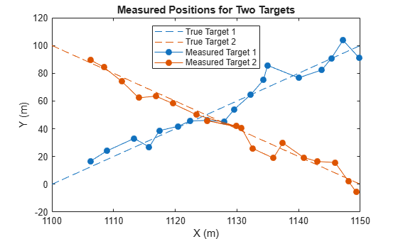
Multiple Targets
The radarDataGenerator can also determine which measurements came from which target. To show this, create a scene, radar, and two targets, each with different trajectories.
% Create radar scenario
scene = radarScenario('UpdateRate',0);

% Place radar on a stationary platform
release(radar);
radar.RangeLimits = [1,1e9];
radarPlat = platform(scene,'Position',radarPos,'Sensors',radar,'Orientation',radarOrientation);

% Create target with specified trajectory
waypoints1 = [1.1e3 0 0; 1.15e3 1e2 0];
trajectory1 = waypointTrajectory('TimeOfArrival',[0; 1e2],'Waypoints',waypoints1);
targetPlat1 = platform(scene,'Trajectory',trajectory1, ...
    'Signatures',{rcsSignature('Pattern',ones(2,2)*10)});

waypoints2 = [1.1e3 1e2 0; 1.15e3 0 0];
trajectory2 = waypointTrajectory('TimeOfArrival',[0; 1e2],'Waypoints',waypoints2);
targetPlat2 = platform(scene,'Trajectory',trajectory2, ...
    'Signatures',{rcsSignature('Pattern',ones(2,2)*10)});

% IMPORTANT: Allows the radarDataGenerator to use the RCS of the target platform
radar.Profiles = platformProfiles(scene);
Run the simulation and plot the detections for each target.
rng('default')
allTracks = [];
while scene.advance
    tgtPoses = targetPoses(radarPlat);
    ins = pose(radarPlat);
    tracks =radar(tgtPoses,ins,scene.SimulationTime);

    % Compile any new track data
    allTracks = [allTracks;tracks];
end

ids = [allTracks.TrackID];
track1 = allTracks(ids == 1);
track2 = allTracks(ids == 2);

target1Locations = arrayfun(@(x) [x.State(1),x.State(3)] ,track1 ,'UniformOutput' ,false);
target1Locations = cell2mat(target1Locations);

target2Locations = arrayfun(@(x) [x.State(1),x.State(3)] ,track2 ,'UniformOutput' ,false);
target2Locations = cell2mat(target2Locations);

figure;
plot(waypoints1(:,1),waypoints1(:,2),'--','Color',colors(1,:),'DisplayName','True Target 1')
hold on
plot(waypoints2(:,1),waypoints2(:,2),'--','DisplayName','True Target 2')
plot(target1Locations(:,1),target1Locations(:,2),'.-','MarkerSize',20,'Color',colors(1,:),'DisplayName','Measured Target 1')
plot(target2Locations(:,1),target2Locations(:,2),'.-','MarkerSize',20,'Color',colors(2,:),'DisplayName','Measured Target 2')
legend('Location','north');

xlabel('X (m)')
ylabel('Y (m)')
title('Measured Positions for Two Targets')
Helper Functions
function helperPlotCov(track,color)
    theta = 0:0.01:2*pi;
    covMat = track.StateCovariance([1,3],[1,3]);
    state = track.State([1,3]);
    [evec,eval] = eigs(covMat);
    mag = sqrt(diag(eval)).';
    u = evec(:,1)*mag(1);
    v = evec(:,2)*mag(2);
    x = cos(theta)*u(1) + sin(theta)*v(1);
    y = cos(theta)*u(2) + sin(theta)*v(2);
    plot(x + state(1),y + state(2),'Color',color,'DisplayName','1 \sigma of Covariance');
end

function helperPlotMaxRange(radar)
    r = radar.RangeLimits(2);
    ang=linspace(0,.1,100);
    xp=r*cos(ang);
    yp=r*sin(ang);
    plot(xp,yp,'DisplayName','Max Detectable Range');
end
Scanning
All of the examples thus far have used staring radars. Below, we show examples of four scanning modes. In each of these examples, all radars only scan in the xy-plane (azimuth) but can be extended to include elevation as well. These examples all rely on the radarScenario to advance the radar's look angle at the appropriate rate. More advanced scanning configurations can be found in Simulate a Scanning Radar.
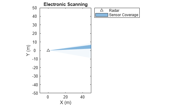
Electronic Scanning
Electronic scanning starts at the minimum coverage limit and progresses to the upper limit in increments equal to the radar's field of view. Once the radar has reached the upper scan limit, the look angle jumps back to the minimum scan limit. Create a radarDataGenerator that scans electronically and use the coveragePlotter to show the look angle and field of view of the radar in a radarScenario.
scene = radarScenario('UpdateRate',0);
figure;
tPlot = theaterPlot('XLim',[-10 50],'YLim',[-50 50],'ZLim',[-100 0]);
title('Electronic Scanning')
radarPlat = platform(scene);
radar = radarDataGenerator(1, ...
    'UpdateRate', .1, ...
    'ScanMode', 'Electronic', ...
    'HasINS', true, ...
    'TargetReportFormat', 'Detections', ...
    'DetectionCoordinates', 'Scenario', ...
    'ElectronicAzimuthLimits',[-10 10], ...
    'FieldOfView',5);
radarPlat.Sensors = radar;
pPlotter = platformPlotter(tPlot,'DisplayName','Radar');
plotPlatform(pPlotter, radarPlat.Position);
covPlotter = coveragePlotter(tPlot,'DisplayName','Sensor Coverage');

ii = 0;
while ii < 100 % run for 100 dwells
    advance(scene);
    config = coverageConfig(radar);
    plotCoverage(covPlotter, config);
    detect(scene);
    pause(.001)
    ii = ii+1;
end
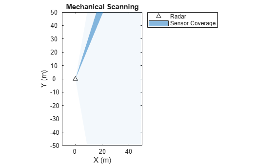
Mechanical Scanning
Unlike electronic scanning, the mechanical scan pattern goes from one scan limit to the other and back to the first without any discontinuities. In other words, there are no jumps from one scan limit to the other. Modify the last radarDataGenerator to make it scan mechanically and create a similar plot as above.
restart(scene)
reset(radar)
radar.ScanMode = "Mechanical";
radar.MechanicalAzimuthLimits = [-80 80];

figure;
tPlot = theaterPlot('XLim',[-10 50],'YLim',[-50 50],'ZLim',[-100 0]);
title('Mechanical Scanning')
pPlotter = platformPlotter(tPlot,'DisplayName','Radar');
plotPlatform(pPlotter, radarPlat.Position);
covPlotter = coveragePlotter(tPlot,'DisplayName','Sensor Coverage');

ii = 0;
while ii < 100 % run for 100 dwells
    advance(scene);
    config = coverageConfig(radar);
    plotCoverage(covPlotter, config);
    detect(scene);
    pause(.001)
    ii = ii+1;
end
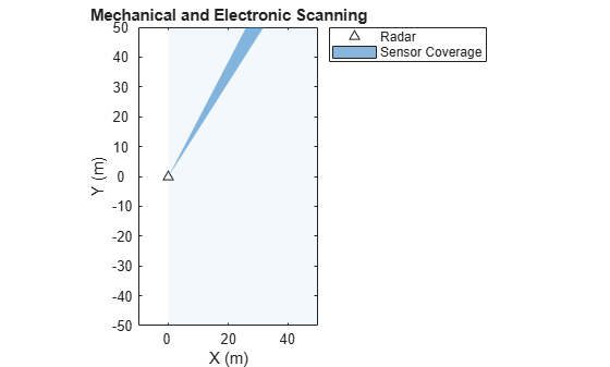
Mechanical and Electronic
The radarDataGenerator can also use both mechanical and electronic scanning. In this mode, the radar continuously scans mechanically based on the mechanical scanning properties defined in the radarDataGenerator. This mode is designed to simulate continuously mechanically scanning radars that use their phased arrays to steer a beam at each mechanical look angle. To implement this, at each mechanical look angle, the radar considers the look angles that are accessible by electronically scanning. It then chooses the look angle that was visited the least recently. Thus, the final look angle at each dwell is the combination of the mechanical angle and the electronic angle.
Modify the radar above to scan in the mode Mechanical and electronic. Then, show the coverage plot just as you did with the other modes.
restart(scene)
reset(radar)
radar.ScanMode = "Mechanical and electronic";

figure;
tPlot = theaterPlot('XLim',[-10 50],'YLim',[-50 50],'ZLim',[-100 0]);
title('Mechanical and Electronic Scanning')
pPlotter = platformPlotter(tPlot,'DisplayName','Radar');
plotPlatform(pPlotter, radarPlat.Position);
covPlotter = coveragePlotter(tPlot,'DisplayName','Sensor Coverage');

ii = 0;
while ii < 100 % run for 100 dwells
    advance(scene);
    config = coverageConfig(radar);
    plotCoverage(covPlotter, config);
    detect(scene);
    pause(.001)
    ii = ii+1;
end
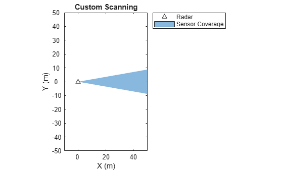
Custom Scanning
Lastly, the radarDataGenerator can also scan in a custom pattern. This mode is great for applications where the radar changes its look angle based on the estimated location of targets or a custom search pattern altogether.
To configure the scanning pattern, define the radar's look angle at each time step. One difference to take note of between the custom mode and the modes discussed thus far is that the field of view property is no longer used. Instead, the beamwidth is determined by the azimuth and elevation resolution.
Define a custom scanning radar that observes 10 degrees per dwell and scans to look angles separated by 30 degrees.
restart(scene)
radar = radarDataGenerator(1, ...
    'UpdateRate', .1, ...
    'ScanMode', 'Custom', ...
    'HasINS', true, ...
    'TargetReportFormat', 'Detections', ...
    'DetectionCoordinates', 'Scenario', ...
    'AzimuthResolution',10);
radarPlat.Sensors = radar;

figure;
tPlot = theaterPlot('XLim',[-10 50],'YLim',[-50 50],'ZLim',[-100 0]);
title('Custom Scanning')
pPlotter = platformPlotter(tPlot,'DisplayName','Radar');
plotPlatform(pPlotter, radarPlat.Position);
covPlotter = coveragePlotter(tPlot,'DisplayName','Sensor Coverage');

ii = 0;
while ii < 100 % run for 100 dwells
    advance(scene);
   radar.LookAngle = mod(30*ii,180)-90; % every 30 degrees
    config = coverageConfig(radar);
    plotCoverage(covPlotter, config);
    detect(scene);
    pause(.001)
    ii = ii+1;
end
Tropospheric Refraction for Workflows Outside of the radarScenario
The radarDataGenerator automatically includes refraction in range and elevation calculations when it is not attached to a radarScenario as a sensor. This single-exponential model of refraction accounts for refraction in the troposphere. The refraction model is described in [1] and [2].
To visualize the impact of refraction on the measured range and elevation, create a staring, monostatic radar with no noise, and no false alarms. Make sure the range limits and field of view are sufficiently large to test the ranges and angles of interest. Also, set the probability of detection to 1 to ensure that the radar detects every target, no matter the range or RCS. Lastly, set the detection coordinates to Sensor spherical so that you can more easily determine the range and elevation biases.
clear
radar = radarDataGenerator(1, 'No Scanning',...
    'HasFalseAlarms',false,...
    'HasElevation',true,...
    'HasNoise',false,...
    'RangeLimits',[1,1e9],...
    'DetectionProbability',1,...
    'DetectionCoordinates','Sensor spherical',...
    'TargetReportFormat','Detections',...
    'FieldOfView',[180,180]);
Create a placeholder target struct with zero velocity. The position will be set in a for-loop later in order to span many ranges and elevation angles.
tgt1 = struct(...
    'PlatformID',1, ...
    'Position', [0 0 0], ...
    'Velocity', [0 0 0]);
Set the test ranges and elevations and use meshgrid to create ordered pairs of the values.
rgTrue = (1e3:1e3:500e3);
elTrue = -(0:15:90);

[elTrues,rgTrues] = meshgrid(elTrue,rgTrue);

% Measured elevations and ranges
elMeas = zeros(numel(rgTrue),numel(elTrue));
rgMeas = zeros(numel(rgTrue),numel(elTrue));

% Loop through positions
for rgIdx = 1:numel(rgTrue)
    for elIdx = 1:numel(elTrue)
        % Set target position
        tgt1.Position = [rgTrue(rgIdx)*cosd(elTrue(elIdx)),0,rgTrue(rgIdx)*sind(elTrue(elIdx))];
        det =radar(tgt1,0); % detect target with radar
        rgMeas(rgIdx,elIdx) = det{1}.Measurement(3);
        elMeas(rgIdx,elIdx) = det{1}.Measurement(2);
    end
end
Refraction causes the measured range to appear farther than the true slant range and the measured elevation to appear higher than the true elevation. Plot these biases with respect to the true slant range.
fig = figure; fig.Position(3:4) = [1024 640];
tl = tiledlayout("vertical","Parent",fig);
title(tl,"Modified Single Exponential Atmospheric Refraction Bias Model")

% Range bias
ax1 = nexttile(tl);
hold(ax1,"on");
plot(ax1,rgTrues/1e3,rgMeas-rgTrues);
xlabel(ax1,"True Slant Range (km)");
ylabel(ax1,"Slant Range Bias (m)");
title(ax1,"Range Bias");
legStr = sprintf("%g,",elTrues(1,:));
legStr = strsplit(legStr,",");
title(legend(ax1,legStr{1:end-1}),"True Elevation (deg)");
grid(ax1,"on"); grid(ax1,"minor");
ax1.YScale = "log";

% Elevation Bias
ax2 = nexttile(tl);
hold(ax2,"on");
elErr = elMeas-elTrues;
xrgErr = deg2rad(elErr).*rgTrues;
plot(ax2,rgTrue/1e3,abs(xrgErr));
xlabel(ax2,"True Slant Range (km)");
ylabel(ax2,"Elevation Cross-Range Bias (m)");
title(ax2,"Elevation Bias");
legStr = sprintf("%g,",elTrues(1,:));
legStr = strsplit(legStr,",");
title(legend(ax2,legStr{1:end-1}),"True Elevation (deg)");
grid(ax2,"on"); grid(ax2,"minor");
ax2.YScale = "log";
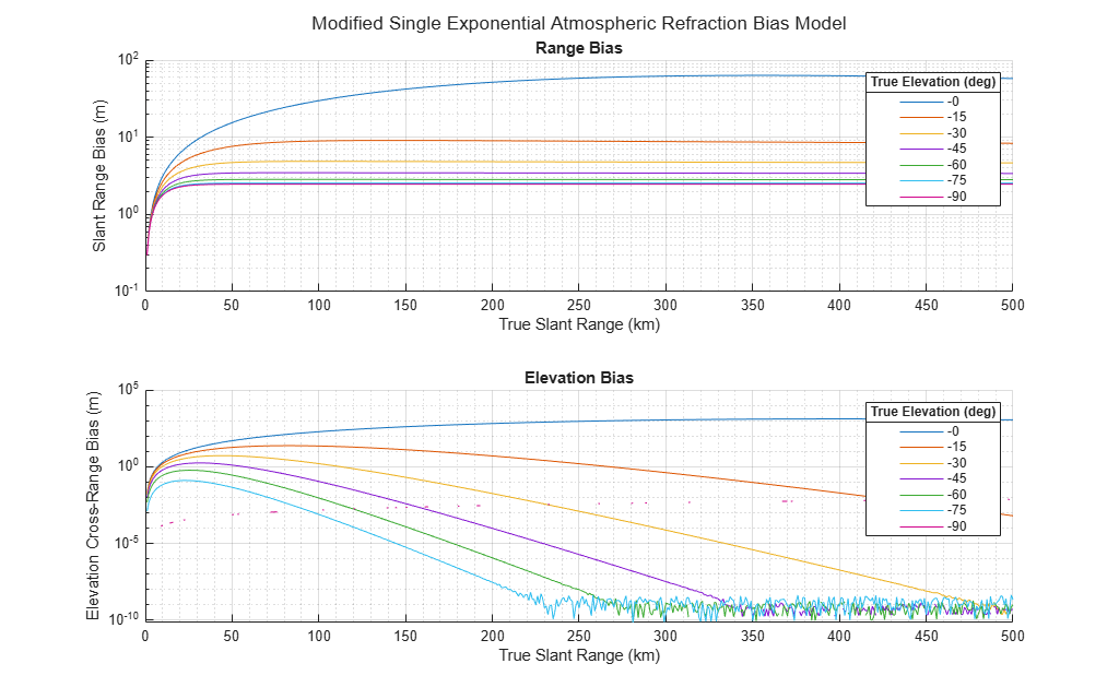
The plot above shows that for low elevation angles, the range and elevation biases are the greatest.
References
[1] Doerry, Armin. "Radar Range Measurements in the Atmosphere," February 2013. https://www.osti.gov/servlets/purl/1088100.
[2] Doerry, Armin . "Earth Curvature and Atmospheric Refraction Effects on Radar Signal Propagation," January 2013. https://www.osti.gov/servlets/purl/1088100.