linearizeOptions

R2026b

Set linearization options

Description

The LinearizeOptions object stores and manages the options for linearization.

Creation

Syntax

options = linearizeOptions

options = linearizeOptions(PropertyName=Value)

Description

options = linearizeOptions returns the default linearization option set.

options = linearizeOptions(PropertyName=Value)sets properties using one or more name-value arguments. For example, linearizeOptions(SampleTime=0.1) sets the sample time for the linearization result to 0.1.

Properties

General Options

LinearizationAlgorithm — Algorithm used for linearization

"blockbyblock" (default) | "numericalpert" | "numericalpert2"

Algorithm used for linearization, specified as one of the following:

• "blockbyblock" — Individually linearize each block in the model, and combine the results to produce the linearization of the specified system.

• "numericalpert" — Full-model numerical-perturbation linearization in which root-level inports and states are perturbed using forward differences; that is, by adding perturbations to the input and state values. This perturbation method is typically faster than the "numericalpert2" method.

• "numericalpert2" — Full-model numerical-perturbation linearization in which root-level inports and states are numerically perturbed using central differences; that is, by perturbing the input and state values in both positive and negative directions. This perturbation method is typically more accurate than the "numericalpert" method.

The numerical perturbation linearization methods ignore linear analysis points set in the model and use root-level inports and outports instead.

Block-by-block linearization has several advantages over full-model numerical perturbation:

• Many Simulink^® blocks have a preprogrammed exact linearization.

• You can use linear analysis points to specify a portion of the model to linearize.

• You can configure blocks to use custom linearizations without affecting your model simulation.

• Structurally nonminimal states are automatically removed.

• You can specify linearizations that include uncertainty (requires Robust Control Toolbox™ software).

• You can obtain detailed diagnostic information about the linearization.

SampleTime — Sample time of linearization result

-1 (default) | 0 | positive scalar

Sample time of linearization result, specified as one of the following:

• -1 — Set the sample time to the least common multiple of the nonzero sample times in the model.

• 0 — Create a continuous-time model.

• Positive scalar — Specify the sample time for discrete-time systems.

UseFullBlockNameLabels — Flag indicating whether to truncate names of I/Os and states

"off" (default) | on/off logical value

Flag indicating whether to truncate names of I/Os and states in the linearized model, specified as one of these values:

• "off", 0, or false — Use truncated names for the I/Os and states in the linearized model.

• "on", 1, or true — Use the full block path to name the I/Os and states in the linearized model.

UseBusSignalLabels — Flag indicating whether to use bus signal channel numbers or names

"off" (default) | on/off logical value

Flag indicating whether to use bus signal channel numbers or names to label the I/Os in the linearized model, specified as one of these values:

• "off", 0, or false — Use bus signal channel numbers to label I/Os on bus signals in the linearized model.

• "on", 1, or true — Use bus signal names to label I/Os on bus signals in the linearized model. Bus signal names appear in the results when the I/O points are located at the output of the following blocks:

  • Root-level inport block containing a bus object

  • Bus creator block

  • Subsystem block whose source traces back to the output of a bus creator block

  • Subsystem block whose source traces back to a root-level inport by passing through only virtual or nonvirtual subsystem boundaries

StoreOffsets — Flag indicating whether to compute linearization offsets

"none" (default) | "struct" | "system"

Flag indicating whether to compute linearization offsets for inputs, outputs, states, and state derivatives or updated states, specified as one of these values:

• "none" — Do not compute linearization offsets.

• "struct" — Return computed linearization offsets in the info output argument of linearize.

• "system" — Store computed linearization offsets in the Offsets property of the linearized system sys. This option is applicable only when sys is an ss or sparss model.

For an example, see Batch Linearize Plant Model and Obtain Linearization Offsets.

You can configure an LPV System block using linearization offsets. For an example, see Approximate Nonlinear Behavior Using Array of LTI Systems

Block-By-Block Algorithm

BlockReduction — Flag indicating whether to omit blocks that are not on the linearization path

"on" (default) | on/off logical value

Flag indicating whether to omit blocks that are not in the linearization path, specified as the comma-separated pair consisting of "BlockReduction" and one of the following:

• "on", 1, or true — Return a linearized model that does not include states from noncontributing linearization paths.

• "off", 0, or false — Return a linearized model that includes all the states of the model.

Dead linearization paths can include:

• Blocks that linearize to zero.

• Switch blocks that are not active along the path.

• Disabled subsystems.

• Signals marked as open-loop linearization points.

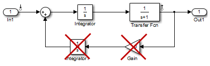
For example, if this flag set to "on", the linearization result of the model shown in the following figure includes only two states. It does not include states from the two blocks outside the linearization path. These states do not appear because these blocks are on a dead linearization path with a block that linearizes to zero (the zero gain block).

This option applies only when LinearizationAlgorithm is "blockbyblock". BlockReduction is always treated as "on" when LinearizationAlgorithm is "numericalpert" or "numericalpert2".

BatchConsistency — Perform state-consistent batch linearization

"off" (default) | on/off logical value

Since R2025a

Flag indicating whether to perform state-consistent reduction for linearized array with uniform state dimension. This means that the software removes only the states and delays that do not contribute to the input-output map for all models in the batch linearization array.

Specify this option as one of these logical on/off values:

• "on", 1, or true — Perform state-consistent reduction.

• "off", 0, or false — Do not perform state-consistent reduction.

For an example, see Obtain Batch Linearization Results with Uniform State Consistency.

IgnoreDiscreteStates — Flag indicating whether to remove discrete-time states

"off" (default) | on/off logical value

Flag indicating whether to remove discrete-time states from the linearization, specified as one of these values:

• "off", 0, or false — Always include discrete-time states.

• "on", 1, or true — Remove discrete states from the linearization. Use this option when performing continuous-time linearization (SampleTime = 0) to accept the D value for all blocks with discrete-time states.

This option applies only when LinearizationAlgorithm is "blockbyblock".

UseExactDelayModel — Flag indicating whether to compute linearization with exact delays

"off" (default) | on/off logical value

Flag indicating whether to compute linearization with exact delays, specified as one of these values:

• "off", 0, or false — Return a linear model with approximate delays.

• "on", 1, or true — Return a linear model with exact delays.

This option applies only when LinearizationAlgorithm is "blockbyblock".

AreParamsTunable — Flag indicating whether to recompile the model when varying parameter values

"on" (default) | on/off logical value

Flag indicating whether to recompile the model when varying parameter values for linearization, specified as one of these values:

• "on", 1, or true — Do not recompile the model when all varying parameters are tunable. If any varying parameters are not tunable, recompile the model for each parameter grid point, and issue a warning message.

• "off", 0, or false — Recompile the model for each parameter grid point. Use this option when you vary the values of nontunable parameters.

For more information about model compilation when you linearize with parameter variation, see Batch Linearization Efficiency When You Vary Parameter Values.

StoreAdvisor — Flag indicating whether to store diagnostic information

"off" (default) | on/off logical value

Flag indicating whether to store diagnostic information during linearization, specified as one of these values:

• "off", 0, or false — Do not store linearization diagnostic information.

• "on", 1, or true — Store linearization diagnostic information.

Linearization commands store and return diagnostic information in a LinearizationAdvisor object. For an example of troubleshooting linearization results using a LinearizationAdvisor object, see Troubleshoot Linearization Results at Command Line.

Numerical Perturbation Algorithm

NumericalPertRel — Numerical perturbation level

1e-5 (default) | positive scalar

Numerical perturbation level, specified as a positive scalar. This option applies only when LinearizationAlgorithm is "numericalpert" or "numericalpert2".

The perturbation levels for the system states are:

$$\text{NumericalPertRel}+{10}^{-3}\times \text{NumericalPertRel}\times \left|x\right|$$

The perturbation levels for the system inputs are:

$$\text{NumericalPertRel}+{10}^{-3}\times \text{NumericalPertRel}\times \left|u\right|$$

You can override these values using the NumericalXPert or NumericalUPert options.

NumericalXPert — State perturbation levels

[] (default) | operating point object

State perturbation levels, specified as an operating point object. This option applies only when LinearizationAlgorithm is "numericalpert" or "numericalpert2".

To set individual perturbation levels for each state:

1. Create an operating point object for the model..

   xPert = operpoint("watertank");

2. Set the state values in the operating point object to the perturbation levels.

   xPert.States(1).x = 2e-3;
   xPert.States(2).x = 3e-3;

3. Set the value of the NumericalXPert option to the operating point object.

   opt = linearizeOptions(LinearizationAlgorithm="numericalpert");
   opt.NumericalXPert = xPert;

If NumericalXPert is empty, [], the linearization algorithm derives the state perturbation levels using NumericalPertRel.

NumericalUPert — Input perturbation levels

[] (default) | operating point object

Input perturbation levels, specified as an operating point object. This option applies only when LinearizationAlgorithm is "numericalpert" or "numericalpert2".

To set individual perturbation levels for each input:

1. Create an operating point object for the model.

   uPert = operpoint("watertank");

2. Set the input values in the operating point object to the perturbation levels.

   uPert.Inputs(1).x = 3e-3;

3. Set the value of the NumericalUPert option to the operating point object.

   opt = linearizeOptions(LinearizationAlgorithm="numericalpert");
   opt.NumericalUPert = uPert;

If NumericalUPert is empty, [], the linearization algorithm derives the input perturbation levels using NumericalPertRel.

Rate Conversion

RateConversionOptions — Rate conversion options for discretization

RateConversionOptions object (default)

Rate conversion options, specified as a RateConversionOptions object with these properties.

Method — Rate conversion method

"zoh" (default) | "tustin" | "prewarp" | "upsampling_zoh" | "upsampling_tustin" | "upsampling_prewarp"

Method used for rate conversion when linearizing a multirate system, specified as one of these values:

• "zoh" — Zero-order hold rate conversion method

• "tustin" — Tustin (bilinear) method

• "prewarp" — Tustin method with frequency prewarp. When you use this method, set the PrewarpFrequency option to the desired prewarp frequency.

• "upsampling_zoh" — Upsample discrete states when possible, and use "zoh" otherwise.

• "upsampling_tustin" — Upsample discrete states when possible, and use "tustin" otherwise.

• "upsampling_prewarp" — Upsample discrete states when possible, and use "prewarp" otherwise. When you use this method, set the PrewarpFrequency option to the desired prewarp frequency.

For more information on rate conversion and linearization of multirate models, see:

• Linearize Multirate Models

• Linearize Models Using Different Rate Conversion Methods

• Continuous-Discrete Conversion Methods

Note

If you use a rate conversion method other than "zoh", the converted states no longer have the same physical meaning as the original states. As a result, the state names in the resulting LTI system change to "?".

This option applies only when LinearizationAlgorithm is "blockbyblock".

Example: options.RateConversionOptions.Method = "tustin";

DelayModeling — Format of modeling extra delays

"state" (default) | "delay"

Since R2025a

Format of modeling extra delays arising from discretization, specified as "delay" or "state". Discretizing models with input or output delays that are fractional multiples of Ts can give rise to additional delays besides the discrete input and output delays. Use this option to specify whether to model these extra delays as internal delays ('"delay") or additional states ("state").

This option is only applicable when UseExactDelayModel is on, or when substituting blocks with models that have delays.

Example: options.RateConversionOptions.DelayModeling = "delay";

PrewarpFrequency — Prewarp frequency

0 (default) | positive scalar

Prewarp frequency in rad/s, specified as a nonnegative scalar. This option applies only when RateConversionMethod is either "prewarp" or "upsampling_prewarp".

Example: options.RateConversionOptions.PrewarpFrequency = 100;

ThiranOrder — Maximum order of Thiran filter for "tustin"and "matched" methods

0 (default) | positive integer

Since R2025a

Maximum order of the Thiran filter used to approximate fractional delays in the "tustin" method. A value of 0 means that discretization rounds fractional delays to the nearest integer multiple of the sample time. If you set this property to a positive integer, discretization uses thiran to approximate fractional delays before discretizing.

For models with fractional delays, the Thiran filters contribute additional internal delays when DelayModeling is set to "delay" and additional states when DelayModeling is set to "state".

This option is only applicable when UseExactDelayModel is on, or when substituting blocks with models that have delays.

Example: options.RateConversionOptions.ThiranOrder = 5;

Object Functions

linearize	Linear approximation of Simulink model or subsystem
slLinearizer	Interface for batch linearization of Simulink models
ulinearize (Robust Control Toolbox)	Linearize Simulink model with Uncertain State Space block

Examples

Create Option Set for Linearization

Create a linearization option set that stores the linearization offsets with the linearized model and instructs linearization not to omit blocks outside the linearization path.

options = linearizeOptions( ...
    BlockReduction="off", ...
    StoreOffsets="system")

options = 
  LinearizeOptions with properties:

    LinearizationAlgorithm: 'blockbyblock'
                SampleTime: -1
    UseFullBlockNameLabels: off
        UseBusSignalLabels: off
              StoreOffsets: 'system'

   Block-by-block algorithm options
            BlockReduction: off
          BatchConsistency: off
      IgnoreDiscreteStates: off
        UseExactDelayModel: off
          AreParamsTunable: on
              StoreAdvisor: off

   Numerical perturbation algorithm options
          NumericalPertRel: 1.0000e-05
            NumericalXPert: []
            NumericalUPert: []

   Rate conversion options (RateConversionOptions)
                    Method: 'zoh'
             DelayModeling: 'state'
          PrewarpFrequency: 10
               ThiranOrder: 0

Additionally, to set the rate conversion method to the Tustin method with prewarping at a frequency of 10 rad/s, use dot notation to set the values of options.

options.RateConversionOptions.Method = "prewarp";
options.RateConversionOptions.PrewarpFrequency = 10

options = 
  LinearizeOptions with properties:

    LinearizationAlgorithm: 'blockbyblock'
                SampleTime: -1
    UseFullBlockNameLabels: off
        UseBusSignalLabels: off
              StoreOffsets: 'system'

   Block-by-block algorithm options
            BlockReduction: off
          BatchConsistency: off
      IgnoreDiscreteStates: off
        UseExactDelayModel: off
          AreParamsTunable: on
              StoreAdvisor: off

   Numerical perturbation algorithm options
          NumericalPertRel: 1.0000e-05
            NumericalXPert: []
            NumericalUPert: []

   Rate conversion options (RateConversionOptions)
                    Method: 'prewarp'
             DelayModeling: 'state'
          PrewarpFrequency: 10
               ThiranOrder: 0

Version History

Introduced in R2013b

R2025a: Improvements to sparse and descriptor state-space linearization, discrete rate conversion, offset handling, and state consistency

The linearization tools available in Simulink Control Design™ software now provide the following enhancements for linearization:

• Sparse linearization — The software can now return a first-order sparse (sparss) model without relying on block substitution for sparse-capable blocks. Previously, you could only perform sparse linearization when BlockReduction option of linearizeOptions and slTunerOptions was set to "on".

• Enhanced rate conversion options — The linearizeOptions and slTunerOptions objects now store the rate conversion related options under the new RateConversionOptions property. Additionally, rate conversion options now include DelayModeling and ThiranOrder. The DelayModeling option allows you to specify whether to model extra delays from discretization as internal delays or additional states. The ThiranOrder option specifies the order of the Thiran filter used to approximate fractional delays in the Tustin discretization. To set these properties, use dot notation:

  opt = linearizeOptions;
  opt.RateConversionOptions.Method = "tustin";
  opt.RateConversionOptions.DelayModeling = "delay";
  opt.RateConversionOptions.ThiranOrder = 3;

• Offset computation and storage — The software now allows you to directly store offsets in the Offsets property of the linearized ss and sparss models using the new value "system" for the option.

  opt = linearizeOptions(StoreOffsets="system")

  Additionally, you can now compute offsets during snapshot linearization. Calculation of offsets during simulation are limited to continuous time blocks and linear discrete time blocks. For example:

  tsnap = 7.5;
  sys = linearize(mdl,io,tsnap,opt);

• Consistent block reduction — When performing batch linearization, you can now use the new BatchConsistency option of linearizeOptions and slTunerOptions to only reduce the states that are reducible for all models in the grid of operating points. In addition, the software maintains this consistency during any rate conversion or delay modeling.

These changes also simplify LPV modeling workflows. Building LPV models in MATLAB^® and Simulink require consistent and uniform state dimensions, delay modeling, and offset handling across the linearization grid. For more information about building LPV models from batch linearization results, see ssInterpolant.

R2025a: linearizeOptions and slTunerOptions: Offset and rate conversion options changed

As a result of improvements to linearization workflows, how you specify options related to offsets and rate conversion in linearizeOptions and slTunerOptions have changed. This table describes the change in the workflow.

Before R2025a	R2025a
Offsets Do not compute linearization offsets. opt.StoreOffsets = "off"; Compute linearization offsets and return as an output argument of linearize. opt.StoreOffsets = "on"; [sys,~,info] = linearize(__,opt); offsets = info.Offsets;	Offsets Do not compute linearization offsets. opt.StoreOffsets = "none"; Compute linearization offsets and return as an output argument of linearize. opt.StoreOffsets = "struct"; [sys,~,info] = linearize(__,opt); offsets = info.Offsets;
Rate conversion Rate conversion method opt.RateConversionMethod = "tustin"; Prewarp frequency opt.PreWarpFreq = 10;	Rate conversion Rate conversion method opt.RateConversionOptions.Method = "tustin"; Prewarp frequency opt.RateConversionOptions.PrewarpFrequency = 10;