evcdf

Extreme value cumulative distribution function

Syntax

p = evcdf(x)

p = evcdf(x,mu,sigma)

[p,pLo,pUp] = evcdf(x,mu,sigma,pCov)

[p,pLo,pUp] = evcdf(x,mu,sigma,pCov,alpha)

[___] = evcdf(___,"upper")

Description

p = evcdf(x) returns the cumulative distribution function (cdf) of the type 1 extreme value distribution (also known as the Gumbel distribution) with a location parameter equal to 0 and a scale parameter equal to 1, evaluated at the values in x. The software returns the cdf for the minimum case. To model the maximum case, call evcdf using the negative of the original values in x, and specify the last input argument as "upper". For more information, see Extreme Value Distribution.

p = evcdf(x,mu,sigma) returns the cdf with the location parameters mu and scale parameters sigma, evaluated at the values in x.

[p,pLo,pUp] = evcdf(x,mu,sigma,pCov) also returns the 95% confidence bounds [pLo,pUp] of p when mu and sigma are estimates. pCov is a 2-by-2 covariance matrix of the estimated parameters.

[p,pLo,pUp] = evcdf(x,mu,sigma,pCov,alpha) specifies the confidence level as 100(1 – alpha)% for the confidence interval [pLo,pUp].

[___] = evcdf(___,"upper") returns the complement of the cdf, evaluated at the values in x, using an algorithm that more accurately computes the extreme upper-tail probabilities. "upper" can follow any of the input argument combinations in the previous syntaxes.

Examples

Compute Type 1 Extreme Value Cumulative Distribution Function

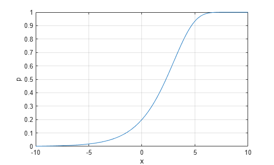
Compute the cumulative distribution function (cdf) for a type 1 extreme value distribution with the location parameter mu=3 and the scale parameter sigma=2.

x = -10:0.1:10;
mu = 3;
sigma = 2;
p = evcdf(x,mu,sigma);

Plot the cdf.

plot(x,p)
grid on
xlabel("x")
ylabel("p")

Confidence Interval of Gumbel cdf Value

Find the maximum likelihood estimates (MLEs) of the type 1 extreme value (Gumbel) distribution parameters, and then find the confidence interval of the corresponding cdf value.

Generate 1000 random numbers from the Gumbel distribution with the location parameter mu=4 and the scale parameter sigma=3.

rng(0,"twister") % For reproducibility
n = 1000; % Number of samples
mu = 4;
sigma = 3;
x = evrnd(mu,sigma,n,1);

Find the MLEs for the Gumbel distribution parameters by using the mle function.

phat = mle(x,Distribution="ev")

phat = 1×2

    4.0806    2.8181

muHat = phat(1);
sigmaHat = phat(2);

Estimate the covariance of the distribution parameters by using the evlike function. The function returns an approximation to the asymptotic covariance matrix if you pass the MLEs and the samples used to estimate the MLEs.

[~,pCov] = evlike(phat,x)

pCov = 2×2

    0.0088   -0.0020
   -0.0020    0.0049

Find the cdf value at 0.5 and its 95% confidence interval.

[p,pLo,pUp] = evcdf(0.5,muHat,sigmaHat,pCov)

p = 
0.2447

pLo = 
0.2237

pUp = 
0.2673

p is the cdf value of the Gumbel distribution with the parameters muHat and sigmaHat. The interval [pLo,pUp] is the 95% confidence interval of the cdf evaluated at 0.5, considering the uncertainty of muHat and sigmaHat using pCov. The 95% confidence interval means the probability that [pLo,pUp] contains the true cdf value is 0.95.

Compute Extreme Upper-Tail Probabilities for Extreme Value Distribution

Determine the probability of sampling a number greater than 5 from the type 1 extreme value distribution with the location parameter mu=1 and scale parameter sigma=1. To determine the probability, calculate the probability of sampling a number less than or equal to 5 and subtract the result from 1.

mu = 1;
sigma = 1;
p1 = 1 - evcdf(5,mu,sigma)

p1 = 
0

The probability of sampling a number less than or equal to 5 is so close to 1 that subtracting the probability from 1 gives 0.

To approximate the extreme upper-tail probability with greater precision, compute the complement of the extreme value cdf directly.

p2 = evcdf(5,1,1,"upper")

p2 = 
1.9423e-24

The output indicates a small probability of sampling a number greater than 5.

Input Arguments

x — Values at which to evaluate extreme value cdf

scalar value | array of scalar values

Values at which to evaluate the extreme value cdf, specified as a scalar value or an array of scalar values.

To evaluate the cdf at multiple values, specify x as an array. To evaluate the cdfs of multiple distributions, specify either mu or sigma (or both) using arrays. If one or more of the input arguments x, mu, and sigma are arrays, then the array sizes must be the same. In this case, evcdf expands each scalar input into a constant array of the same size as the array inputs. Each element in p is the cdf value of the distribution specified by the corresponding elements in mu and sigma, evaluated at the corresponding element in x.

If you specify pCov to compute the confidence interval [pLo,pUp], then x must be a scalar value.

Data Types: single | double

mu — Location parameter

0 (default) | scalar value | array of scalar values

Location parameter, specified as a scalar value or an array of scalar values.

To evaluate the cdf at multiple values, specify x as an array. To evaluate the cdfs of multiple distributions, specify either mu or sigma (or both) using arrays. If one or more of the input arguments x, mu, and sigma are arrays, then the array sizes must be the same. In this case, evcdf expands each scalar input into a constant array of the same size as the array inputs. Each element in p is the cdf value of the distribution specified by the corresponding elements in mu and sigma, evaluated at the corresponding element in x.

If you specify pCov to compute the confidence interval [pLo,pUp], then mu must be a scalar value.

Data Types: single | double

sigma — Scale parameter

1 (default) | positive scalar value | array of positive scalar values

Scale parameter, specified as a positive scalar value or an array of positive scalar values.

To evaluate the cdf at multiple values, specify x as an array. To evaluate the cdfs of multiple distributions, specify either mu or sigma (or both) using arrays. If one or more of the input arguments x, mu, and sigma are arrays, then the array sizes must be the same. In this case, evcdf expands each scalar input into a constant array of the same size as the array inputs. Each element in p is the cdf value of the distribution specified by the corresponding elements in mu and sigma, evaluated at the corresponding element in x.

If you specify pCov to compute the confidence interval [pLo,pUp], then sigma must be a scalar value.

Data Types: single | double

pCov — Covariance of estimates

2-by-2 numeric matrix

Covariance of the estimates mu and sigma, specified as a 2-by-2 numeric matrix.

If you specify pCov to compute the confidence interval [pLo,pUp], then x, mu, and sigma must be scalar values.

You can estimate mu and sigma by using mle, and estimate the covariance of mu and sigma by using evlike. For an example, see Confidence Interval of Gumbel cdf Value.

Data Types: single | double

alpha — Significance level

0.05 (default) | scalar in the range (0,1)

Significance level for the confidence interval, specified as a scalar in the range (0,1). The confidence level is 100(1 – alpha)%, where alpha is the probability that the confidence interval does not contain the true value.

Data Types: single | double

Output Arguments

p — Type 1 extreme value cdf values

scalar value | array of scalar values

Type 1 extreme value cdf values, returned as a scalar value or an array of scalar values. p is the same size as x, mu, and sigma after any necessary scalar expansion. Each element in p is the cdf value of the distribution specified by the corresponding elements in mu and sigma, evaluated at the corresponding element in x.

pLo — Lower confidence bound for p

scalar value | array of scalar values

Lower confidence bound for p, returned as a scalar value or an array of scalar values. pLo is the same size as p.

pUp — Upper confidence bound for p

scalar value | array of scalar values

Upper confidence bound for p, returned as a scalar value or an array of scalar values. pUp is the same size as p.

More About

Type 1 Extreme Value cdf

The type 1 extreme value (Gumbel) cdf in the minimum case is

$$p=F\left(x|\mu ,\sigma \right)=1-\exp \left(-\exp \left(\frac{x-\mu }{\sigma }\right)\right)$$

The result p is the probability that a single observation from a type 1 extreme value distribution with the location parameter μ and scale parameter σ will fall in the interval [–Inf x].

This version of the distribution is suitable for modeling minima. You can use the mirror image of this distribution to model maxima by negating x and subtracting the resulting distribution values from 1. If x has a Weibull distribution, then X = log(x) has the type 1 extreme value distribution. See Extreme Value Distribution for more details.

Algorithms

The function computes confidence bounds for p using a normal approximation to the distribution of the estimate

$$\frac{X-\widehat{\mu }}{\widehat{\sigma }}$$

and then transforming those bounds to the scale of the output p. The computed bounds give approximately the intended confidence level when you estimate mu, sigma, and pcov from large samples. When you use smaller samples, other methods of computing the confidence bounds might be more accurate.

Alternative Functionality

• evcdf is a function specific to the extreme value distribution. Statistics and Machine Learning Toolbox™ also offers the generic function cdf, which supports various probability distributions. To use cdf, create an ExtremeValueDistribution probability distribution object and pass the object as an input argument or specify the probability distribution name and its parameters. Note that the distribution-specific function evcdf is faster than the generic function cdf.

• Use the Probability Distribution Function Tool to create an interactive plot of the cumulative distribution function (cdf) or probability density function (pdf) for a probability distribution.

References

[1] Crowder, Martin J., ed. Statistical Analysis of Reliability Data. Reprinted. London: Chapman & Hall, 1995.

[2] Lawless, J. F. Statistical Models and Methods for Lifetime Data. Hoboken, NJ: Wiley-Interscience, 2002.

[3] Meeker, W. Q., and L. A. Escobar. Statistical Methods for Reliability Data. Hoboken, NJ: John Wiley & Sons, Inc., 1998.

Extended Capabilities

C/C++ Code Generation
Generate C and C++ code using MATLAB® Coder™.

GPU Arrays

Accelerate code by running on a graphics processing unit (GPU) using Parallel Computing Toolbox™.

This function fully supports GPU arrays. For more information, see Run MATLAB Functions on a GPU (Parallel Computing Toolbox).

Version History

Introduced before R2006a