Green Hydrogen Production in Microgrids - MATLAB & Simulink
Video Player is loading.
Current Time 0:00
Duration 42:58
Loaded: 0.38%
Stream Type LIVE
Remaining Time 42:58
 
1x
  • Chapters
  • descriptions off, selected
  • captions off, selected
  • en (Main), selected
    Video length is 42:58

    Green Hydrogen Production in Microgrids

    Overview

    Production of green hydrogen by electrolysis is identified as an enabler for electrified transportation and fossil-free industrial processes. Electric power harvested from renewable energy sources (wind, solar) is converted into hydrogen gas. Despite the undoubted potential, planning, design and operation of electrolysis plants present several challenges. Join this MathWorks presentation to discover how physical system simulation can empower R&D engineering tasks ranging from performance analyses and controls development to techno-economic studies and deployment.

    Highlights

    • Physical multi-domain modeling and simulation
    • Trade-off model fidelity versus simulation objective
    • Micro-grid integration and techno-economic analysis
    • Power electronics control design
    • Options for sharing models such as Apps, FMU
    • Please allow approximately 60 minutes to attend the presentation and Q&A session.

    About the Presenters

    Juan Sagarduy is a senior application engineer in the control design and automation field. His specific focus is physical multidomain modeling and simulation. In his role, Juan provides technical expertise for successful adoption of plant modeling tools (Simscape™ platform) for model-based development. In recent years, he has led several initiatives within Electrification for the Nordic region. Before joining MathWorks in 2011, Juan worked at the ABB Corporate Research Centre (Västerås, Sweden) in electrical machines and motion control projects. Juan holds an M.S. degree in industrial engineering (Bilbao, Spain) and a Ph.D. in electrical engineering from Cardiff University in the UK.

    Tadele Shiferaw is an application engineer at MathWorks Benelux based in Eindhoven. He coordinates the engagement on power electronics design and control with customers from multiple industries within the Benelux area. His technical focus areas include physical modeling of systems, controller design, systems engineering and hardware-in-the loop simulations. Tadele completed a graduate study in control systems and a Ph.D. on controller design for safe robotic manipulation at University of Twente in the Netherlands.

    Recorded: 30 Mar 2022

    Good morning, everybody, and welcome to our seminar today entitled, Green Hydrogen Production in Microgrids. My name is Juan Sagarduy, I'm the application engineer at The MathWorks Nordic office in Sweden. Together with me, I have my colleague Tadele who will introduce himself a bit later on.

    So this event today is the first thing, hydrogen event series from MathWorks. So event number two will focus on hydrogen transfer from tank to fuel cell, and then event three will be focusing on e-mobility with fuel cells. So the agenda that I would like to propose to you today consists of three parts. I will start with a green hydrogen production through electrolysis. I will focus on energy conversion from wind to gas.

    My colleague Tadele will take over and tackle techno-economic analysis with physical models. The user case will be photovoltaic to gas. We will touch upon how the MathWorks chain can empower collaborative R&D with deployment possibilities and MATLAB applications. We will reserve a bit of time to sum up, and then give you some follow-up opportunities.

    So let's get started then. So the chemical process to produce hydrogen is called electrolysis. So water and electrical energy are converted into hydrogen and oxygen. So if the electrical energy to produce hydrogen comes from renewable energy sources like wind and sun, then the hydrogen produced is labeled as green.

    So this technology has got many advantages when it comes to enabling electrification-- so sustainability and versatility, the two of them. But it does have quite a few challenges associated to it. And those are related to high energy consumption, the safety in managing hydrogen, and the high cost. We believe that simulation-based R&D can definitely mitigate the risk and then put you on a path to success.

    So it would start with a microgrid that is solar based. So those are the elements that you're going to find-- photovoltaic panels, energy storage units, often with a battery, and then the electrolyzer, whereby an electrical energy will be resulting in hydrogen. So Tadele will focus on that particular type of microgrid, and then both Tadele and I will use, again, across the value of the Simscape multi-domain platform to green hydrogen production.

    In my case, I will be using a microwave wind-based, then the photovoltaic panels are then replaced by your generator, basically. So when it comes to green hydrogen production from renewables, the ability to import data from wind or sun into models is very important. And there are many available sources online that you can find. So in this case, you see a wind speed trace for almost one day from Inverness in Scotland. And that can be definitely very well done in MATLAB, and then reused by Simulink and Simscape models.

    So if you have now made the choice of using simulation for your development in green hydrogen, then of course fidelity is going to be a critical element into that. If you are focusing on embedded developmental component-focused tasks, then your target is going to be milliseconds or microseconds. You will naturally high fidelity models.

    If you are, on the other hand, interested in assessing key system performance, and the phenomena that lasts over seconds or minutes, then medium fidelity will make a lot of sense. And then last but not least, if your goal is, on the other hand, to assess the feasibility of green hydrogen-- you are looking into a wide calculation for months and years-- then very agile models with the lowest fidelity will be definitely the right choice for you.

    So let's say we focus on the electrolysis unit to start with. So I'd like to bring your attention to what has precisely come in 2022a release. So we have an open Simscape implementation of an electrolyzer, and that captures the thermodynamics really in detail. So you are very welcome to access and use, if that is the focus that you have.

    But then if you are, once again, a bit more focused on system level analysis, on child simulations, you want to understand the technology and maybe start to see different opportunities, to work with it. Then electrolyzer block-- an example is Simscape Electrical also in 22a, are definitely very suitable for you. And this is going to be the case for the seminar. We're going to use that electrolyzer block.

    So energy conversion, wind to gas, I think it's worth mentioning that power electronics are going to be key in converting mechanical energy all the way to gas. So what is it that happens? So a generator is mechanical power, and then electrical power that goes into the electrolyzer. Then in between, you will have power electronics.

    So elements in the power electronics chain, they will start with the generator itself, DC or AC type, induction versus synchronous. Then DC-DC converters-- different elements will have their own DC-DC converter, electrolyzer, and battery. And then if you are using a three phase AC generator in your electrolysis unit, or that unit is grid-connected, then you will need--

    So let's get started with a high fidelity view on green hydrogen production, embedded development, and component analysis. So what are the challenges that we are going to meet on the physical unit level? So those are going to be related to the components themselves and how we regulate them.

    So the electrolyzer, being a core element into that system, energy storage-- often a battery. And then the BMS, battery management system, needs to interact with the rest of the elements in the grid. Power converters-- they need fault management and grid connection algorithms, regulation of power, and even cooling. And then the generator.

    High fidelity models will prove also very useful for digital twin development. Physical models of high fidelity can be used for synthesizing data of degradation and anomalous behavior. Then by generating that data, we can identify features that can be assisting us in prognostics development. So that is predictive maintenance or estimating remaining lifetime for a given component, for instance.

    So if we zoom in a bit into energy conversion-- so we can say that the Simscape Electrical does give you a phenomenal library with universal machine models that will make the modeling processing pretty quick. If you were to reduce electromagnetic design data, you can do it with the two blocks that you see on the bottom of the screen as well. A detailed DC-DC converter can be assembled from discrete elements like diodes, N-channel MOSFETs, or ITVPs. They can even have a thermal option.

    A similar reflection applies to AC to DC converters. So we can use pre-built components where we can make a choice on what particular switch we want to use. But of course, you can compose your own converter with discrete elements as we saw before. In the end, you will be able to capture high frequency phenomena due to pulse width modulation in the converter.

    So it's important to emphasize that different levels of fidelity can and will coexist in models along the development cycle. So in this case, high fidelity on the generator side, and then medium fidelity on the electrolyzer, on the low side. And that makes perfect sense. Often fidelity is added gradually, and it's very seldom that you start with a high fidelity model for each one of the components. Rather, you add that step by step.

    So this video is going to illustrate the first case of a standalone electrolyzer with high fidelity. So let's get started. So first, an overview of the architecture of the model with all the elements that you recognize. So the permanent magnet, the generator, with all the different parameters that are needed. Then a signal of speed-- this continues, applied onto the shaft.

    The control unit with a field oriented control algorithm for the generator. See the architecture without running the loop. The outer loop will regulate the DC link voltage and generate current reference. Then the inner controller will regulate the current and generate voltage references. Then finally the full suite modulation is also given by the tool. You have different options to customize your own PWM sampling modes in the-- so.

    With that, let's get some results of current, electrolyzer, and generator. When that speed is applied, voltage, absorbed electrical power, DC link and voltage. And then energy consumption per kilogram of hydrogen, and then the estimated hydrogen produced for one day.

    So a brief visual recap for you on the permanent magnet generator control that we saw. The thing I like to emphasize that simulation, and desktop simulation in particular, is a powerful validation method for your algorithms. But don't forget that with automatic code generation is Simulink, it will be able to obtain embedded code for those algorithms to almost any embedded device that you can think of. That will accelerate your development significantly.

    Now let's look into the second case. In this case, the electrolyzer is not going to be standalone, but they're connected to the grid. And so in this case, what we are interested in is to see how the electrolyzer reacts to a change of frequency in the grid. So our phase locked loop, that detects the frequency and then uses that for control purposes.

    Then a transient is observed in the generator currents. Logically, the amplitude and the duration of that transient should be limited in time if the controller is doing a good job. So Simscape Electrical does give you the possibility to do harmonic or FFT analysis. In this case, we're going to do harmonic analysis of a current 15 cycles after the transient.

    So results can be given as a bar diagram, or as a list of numerical values. Those can be exported through MATLAB to any other environment like Excel. But if we were to set the frequency to the actual frequency, 50.4, then we will see that the THD will go down from 18 to a value of 9%. So currents were not as distorted as we thought they were.

    So a visual recap on what we saw in the video and the use of a PLL to detect a great frequency change. And then harmonic analysis-- harmonic analysis is a powerful method that allows energy optimization and prognosis development. The harmonics in current sub-voltages bear information on degradation and anomalous behavior. And those can be used for predictive maintenance purposes, or for estimating the remaining useful lifetime for elements in--

    So last in this first part-- key performance system assessment with a medium fidelity. So what other challenges that we expect at the system level? I think in my opinion, those fall down into two categories-- plant and algorithmic design related.

    So for the plant, the first question to ask yourself is, of course, what is the best concept to produce green hydrogen? Is it going to be AC versus DC generation, if we are going for wind? Or grid versus remote? Is wind or solar the best choice, or do you want to combine both?

    How can the requirements for the different components be met? So the size of those components, the integration, the cost. And then even the scalability of your concept, and that is going to become very, very important if you are aiming at having a serial production of electrolysis.

    Then model-based design will, of course, be instrumental in making that even more effective and rewarding. And then, do you really understand the energy balances in your system? A complex multi-domain system with many different phenomena to consider.

    From an algorithmic point of view, you can pick first. OK, how can I architect the supervisory logic so that it accounts for all the different important functions-- energy storage contribution, the asset management, selection of the right sources. And then also important, how can you set up relevant set points meeting very different circumstances-- history, meteorological conditions? What is the right number of active units that you want to have in each situation?

    So if we go back to energy conversion for a little while, then the machine models that were going to use in this type of work are going to be focusing more on energy flow rather than machine control. DC-DC converters are going to be modular in average. So those can be controlled with a duty cycle, current-to-voltage reference. And they account for losses, and then they are going to be fast to simulate, so a perfect choice for us.

    So just to make that a bit more graphical, a video will be shown now on how system assessment can be done in this wind-based microgrid. So let's get started with a brief overview of the system. So the DC generator with the mechanical parts and the electrical part. Then we have the energy storage with a dynamic battery.

    We have a supervisory logic, where we set up switch logic, electrolysis, and battery set points. It's worth mentioning that we have two ways of regulating that system, energy or voltage based. We will come back to that later. DC-DC converter controlled with a voltage reference, and then accounting for losses, then our electrolyzer multi-domain.

    So with that said, then we get some important KPIs from the system-- current, voltage, hydrogen mass produced, and energy consumption. So in this case with a voltage-based algorithm, production is around 38 kilograms of hydrogen. The battery charge ends up at 50%.

    What will happen if we use the energy-based method instead? Hydrogen production goes up significantly to 48 kilograms. Here we can see a trace of the currents, generator, electrolyzer, and the battery. And the battery-- notice that it recharges itself at the specific point in the run.

    What if we reduce the contribution of the energy storage? So then logically, we lose out on hydrogen produced but the battery retains more charge. It goes down only to 65%.

    So just a brief recap on the results of in the simulation. So we can draw two conclusions here. The energy-based method is more aggressive. It allows us to produce more hydrogen, but at the same time, the mean current in the generator is a lot higher, which means that the lifetime of that generator will be lower if we use it in that way. Then a significant impact of course of the contribution of the battery as well, on the outcome in terms of hydrogen.

    So just to wrap up what will be in the end-- the insights or the information that you are expecting from a system assessment. So those would be expected hydrogen production, water consumption. What is the algorithm or the energy management solution that makes sense, and in which conditions? How intensely do you want to use the physical assets?

    Energy storage based on a given capacity and size. What are the expected duty regimes that you would-- what is the contribution and the impact on the outcome of hydrogen as well? Just keep in mind that those KPIs will end up affecting and determining the planning of operations like collecting, replacing, and maintaining. And those will be having a major impact on the workforce and the cost-- so basically how you run the green hydrogen plant.

    So with that said, I'd like to hand over to Tadele who will introduce techno-economic analysis. OK. With that said, I'd like to hand over to my colleague Tadele, who will introduce you to techno-economic analysis with Simscape and Simulink. Take it away, Tadele.

    Hello, everyone. My name is Tadele Shiferaw, and I'm part of the application engineering team at MathWorks, working from our office in the Netherlands. We are continuing our discussion on green hydrogen production. And in this session, I will focus on how we can perform techno-economic analysis using models and the power of simulation. For the discussion, I will consider a use case where solar energy is used as the main renewable source for our green hydrogen production.

    So let's start with a definition. What is techno-economic analysis? I think the name is self-descriptive. And in short, it is an analytical approach that introduces economic aspects like cost and revenue into applied technologies like energy, petroleum, bioprocessing, and et cetera. In most scenarios, a techno-economic analysis relies on a software model to calculate estimates of capital or operational costs, using inputs from either technical or non-technical financial data.

    As we explore the concept, we'll consider an example techno-economic analysis for setting up a green hydrogen production from solar energy at 242 different locations. Using our analysis, we'll answer typical questions like, which locations have the highest or the lowest energy? Or which of those 242 locations have the highest and the lowest grid cost?

    As I mentioned earlier, a model is the basis of techno-economic analysis. And in the case of solar powered green hydrogen production, we need to have a model that includes three important components-- the solar arrays, the storage battery, and the electrolyzer. If you look at the system, it's exactly similar to the one shown by Juan earlier. But in our case, we have replaced the wind turbines with solar arrays.

    Here I have a complete model of the system in Simulink. So let me switch to MATLAB and run some simulations. Here I have a complete system model of solar powered green hydrogen production, with the solar array, the energy battery, and electrolyzer. And if you look at the parameter which is defined as a stop time, I'm running a full three-day simulation in this scenario.

    One thing you will immediately observe is that the simulation is fast and that I'm able to run a full three-day simulation in less than 10 seconds. I'm also able to capture some important measurements, so I can inspect what happened during this three-day simulation scenario.

    So I can use my data inspector to look at some signals. For example, let's start with the power which was generated from the solar arrays. So here, you can see that there were these three daily peaks, basically highlighting peak power during the daytime, and no power generated during the night times. And let's compare that against the power which was consumed by the electrolyzer, for example.

    Here in pink, you can see the power consumed by the electrolyzer. And then for example, at some instance where there is no power which is generated by the solar panel, the electrolyzer was consuming power. And as you might expect, that actually came from the energy which was stored in the battery.

    We can also look at some other parameters. For example, the amount of hydrogen that was captured during those three-day simulations, and then also the amount of water, for example, consumed to generate that hydrogen. With this complete system model available, we can make modifications to each of the components and try out a number of different scenarios that could likely happen in the actual system.

    Looking at the example model that I have just shown, a question that might pop up in your mind is, how was this model developed? Well, one thing to clarify, is that it was not built in one go. In fact, we used standard systems engineering approaches and modeling best practices to incrementally build it up.

    As we are building a complex system model, the standard workflow that we recommend is that first, start with identifying standalone components, choose the right fidelity to model those individual components, use simulation to understand their behavior in more detail, and then finally test and verify them before interconnecting them into a larger system model. One of the components making up our system is a storage battery, and we can use our physical modeling language, Simscape, to model the battery as its equivalent circuit, or use a complete standard model library block for modeling the complete battery.

    Let me switch to MATLAB and show you an example model to test the performance of a model battery. In this model, there are two separate electrical circuits with different implementations of a battery, and both connected to a current load. The two battery models are parameterized identically. And since they are connected to a similar load, a simulation run will give us an equivalent result from the two separate circuits.

    If we compare modeling the battery using an equivalent circuit or a standalone component, one advantage of using these out of the box complete library blocks is that even though the system is a single block, it might have multiple implementations under it. For example in this case, we can enable a thermal port of the battery. So that in addition to the electrical behavior, we can also investigate the thermal behavior of the battery during a simulation.

    If you are interested in a higher fidelity model of the battery, we can represent the parameters as a lookup table to capture parameter variations due to changes in ambient conditions, like temperature or the state of charge. Another important step in modeling batteries is a parameter estimation, where we used experimental data and optimization workflows so that we can make sure the model behaves exactly similar to the experimental data. If you want to know more about the standard approach on modeling batteries using Simulink and Simscape, please feel free to check out the URL below in this slide.

    The second building block in our system is a solar array that we can model separately, and verify its performance via simulation. Let's switch to MATLAB and explore the model of the solar array. Here I have electrical model of a solar array connected to a load. And I can use this model to run multiple simulations to validate the performance of the solar arrays.

    If I explore what's under the hood, I can identify three main components-- the solar cell, and two additional extending components here. The major component, the solar cell, is the block that converts the irradiance or the power from the sun into electrical energy that flows through the rest of the system. While we are defining the cell behavior here in the configuration, we can also define how a number of these cells could be connected either in series or in parallel to create a panel or an array configuration.

    While this manual parameterization is a possibility here, there is also an option to actually select a manufacturer, and then also a part number. So that there is an automatic parameterization based on the data obtained from manufacturer's datasheet. Once we parameterize the solar cell, we have to extend it with additional components, MPPT and a boost converter that we'll discuss short.

    And then finally, connected to a load so that you can create a performance simulation of a system. Here in this case, I'm running a full simulation for 24 hours using the solar cell. And then I'm also capturing important measurements that I can inspect afterwards. For example, I can check the maximum power that I was able to generate from the system, and then the power that was consumed by the grid, which was obviously less than the solar power. Then I can also look at the voltage and the current that was produced from the solar cells.

    The reason why we have those two additional components, the MPPT and the power converter connected to the solar cell, is because of its special characteristics captured in this IPV curve. The IPV curve, which shows the output voltage versus the output current and the output power, shows that the current deteriorates sharply after a certain threshold voltage. That means that the power gradually increases towards a higher maximum point, and then also gradually declines.

    If we need a very efficient operation of the solar cell, then it means that we have to drive the system to operate at this maximum peak operating point. And one thing to note here is that, because of changes in ambient conditions like temperature or the solar irradiance, this whole curve could shift up and down or left and right. So it means if you need a continuous operation at that efficient point, we have to continuously keep track of where the maximum power point is, and guarantee that we are driving the solar cell at that operating point.

    The whole operation of this maximum power point tracking is implemented by using a concept of impedance matching. Impedance matching is a standard electrical engineering concept where, if you connect a source to a load, maximum power is consumed by the load when the impedance of the load is equivalent to the impedance of the source. So this ideology is applied to design the MPPT algorithm, and that is demonstrated by a model here.

    This model contains two different system implementations that I want to compare using a simulation. Both systems contain a constant DC source, and then they have a similar impedance implemented as a resistor. Both systems also contain a variable impedance load implemented as a variable voltage load here and here. You can see that the main difference between those two systems is, the second system contains an MPPT algorithm implementation together with a back boost converter, so that we deliver maximum power to the load irrespective of its impedance.

    So let's run the simulation here and then compare the power delivered to the load in both scenarios. So the simulation is complete. I can inspect what happened there. So for example on the first case, I can look at the power. And then you see that the power was varying, and it varies depending on the impedance of the load.

    On the second case, I can look at the power consumed. And then you see that the power almost maintains constant value of around 100 watts, which was also delivered at 100 watts, throughout the full simulation cycle. And then if you want to check the second case, you see that the variable voltage on the load side, which means there was a variable impedance also implemented on the second side. But irrespective of the impedance side on the load, we were able to deliver this maximum 100 watt output on the second circuit versus the first one. So that was the value of the MPPT algorithm together with the converter.

    The last major component in our green hydrogen production system is the electrolyzer, which converts water into hydrogen using electricity. Let's explore the model and run some simulations to understand how it operates. Here is a standalone model of the electrolyzer connected to a standard voltage source. I can run multiple simulations with different input voltage sources, for example to understand its detail behavior.

    Let's look at how the electrolyzer is implemented in detail. One thing we can see is that this model is constructed from components that span a number of engineering disciplines. And it's indicated by the different colors that are used in the model here. For example, we can see the electrical domain here in blue, the thermal liquid domain here in light orange, and also a purple color indicating here the gas domain.

    Once the detail electrolyzer is implemented, then we can run simulations to understand and investigate its detailed operational performance. For example, we can use our data in this picture of the simulation to look at the amount of hydrogen that we were able to capture for a given input voltage, and then run multiple simulations to compare how much performance we can get for increasing or decreasing the input voltages. Once the three main components are modeled and verified separately using simulation, then we can start integrating them towards creating a complete system model.

    Once we have the system model, we can run simulations to understand and evaluate the operational performance of the system. If you remember in the beginning, I said our objective was to do a techno-economic analysis on setting up green hydrogen production from solar energy on 242 different locations. But so far, the models that we have created were used for purely technical analysis. Can we reuse the models for techno-economic analysis, or is there some special consideration for models that are relevant for techno-economic analysis?

    Well, it turns out that there are some special considerations for models that are used for techno-economic analysis. The first consideration is that the models are executed for a long duration of time, and we are interested in data points at time interval ranging from 1 minute to 1 hour. Compared to, for example, technical analysis that are interested in time intervals of seconds, or even milliseconds and microseconds, these techno-economic analysis models have a longer duration time, and then also longer time intervals for the models.

    A second important consideration is that they rely on steady state operations on those specific time intervals. This means that they are not interested in the dynamics that happens between two different time intervals. And for that, we use a quasi-steady state simulation, which assumes that the system reaches at a steady state during those specific time intervals of interest.

    The quasi-steady state simulation is implemented by replacing components with the reduced order model equivalent. And this reduced order model is realized by using a lookup table that captures quasi-steady state values at desired time intervals. For example, in this reduced order model of a solar cell, the detailed dynamics is replaced by three different lookup tables that capture the output voltage, the output impedance, and the maximum power point tracking implementation output as a duty cycle for input into the back boost converter. And this way, we'll have a quasi-steady state simulation possible with these kind of models.

    Once we have replaced other components like the energy storage, and also the grid with the reduced order model equivalent, then we can create a complete system model that's really for techno-economic analysis. The input to our model are two things-- the irradiance of that specific location and then the electricity cost at that location. Once we have these two as an input, then we can run multiple simulations for those 242 locations, to understand and answer these important two questions-- the highest and lowest grid cost, and the highest and lowest solar energy captured from the system.

    A full year irradiance data for the 242 locations in North America was captured from National Renewable Energy Laboratory. The data not only contains the solar irradiance, it also contains other information relevant for renewable energy study, such as wind speed and temperature. And for the electricity price data, a representative one day data per location was used, and it was simply repeated 365 times to calculate the cost for a given year.

    With both input data available for all locations, we can make use of parallelization to speed up simulation for the 242 different locations. With such an option enabled, we are able to run the simulation in less than 10 minutes, and are able to answer the four questions that we started with. For example, we are able to find out the lowest grid cost was at Phoenix Sky Harbor International Airport, and the highest solar resource was available at Daggett Barstow Airport. There were also the highest grid cost observed at Quillayute State Airport, and the lowest solar resource also captured at a similar location.

    So in total, we were able to simulate 242 years in less than 10 minutes, and answer our techno-economic question. Both me and Juan have shown you different ways that we can use modeling and simulation to perform purely technical, and also techno-economic analysis. But it is important to note that the development and the utilization of a model is offered in a collaborative way. That is, members of a team will develop a model, and other members within the team will reuse the model to improve efficiency and support collaborative workflow.

    Let's see what are the different options that we can collaborate using solutions from MathWorks. Starting from our two main products, MATLAB and Simulink, you can convert algorithms and applications which are developed in these platforms into an embedded target using our coder solutions. With these hardware independent solution, you can target microcontrollers using our C, C++ code generation, FPJ is using our HDF code generation, PLC is using our structured code generation, and then finally GPU is using our Cuda coordination tools.

    We can also make use of our compiler workflows to deploy our applications and algorithms on different platforms, ranging from a dedicated standalone execution all the way up to integration into a cloud-based enterprise IT system. To highlight a few of the deployment options-- for example, we have a standalone application where we create an executable that runs on a local dedicated PC. We also have an option to create a web app that can be accessed through a browser, and able to run without any installation of MATLAB in the browser.

    The third option is, we can create a service API where we integrate MATLAB application or algorithm as part of our integrated IT system. The final option is, we can export our models as a functional markup unit, FMUs, to be integrated into third party FMI compatible tools. Now, let me hand it back to Juan for some concluding remarks.

    Thank you, Tadele. Good job. So it's now time to wrap up and with some conclusions and follow-up opportunities. So we could see today that MATLAB and Simulink Simscape multi-domain platform enables you for green hydrogen production projects.

    Depending on the level of fidelity in your models. You will be able to tackle different tasks along the product cycle. So embedded development or digital twin with high fidelity models, the system assessment and KPI exploration with a medium fidelity-- concept evaluation, energy management, sizing of components. And then commercial feasibility-- analyze long-term prediction with agile models of low fidelity for techno-economic analysis.

    Collaborative research and development becomes a reality with multiple deployment solutions in the MathWorks tool chain. Those will apply at very different parts of your product cycle. So no matter where you work, how it can be gathered, can be shared, and thus enable concurrent engineering in your company, or even collaboration with universities as well.

    So training will enable effective and homogeneous adoption of the tools. Challenging implementation parcels will be solved through consulting. Follow-up opportunities-- presentation materials, including the slide deck, recordings, even bonus material, will be available to all of you after the event. And that will come through an email with a set of links.

    A completed survey is very valuable to us. First, because we are eager to get your feedback on the seminar today. But eventually, we'll want to give you the possibility to share or ask queries on projects, tools, services. And then more importantly, you will be able to request the specific model. So by filling in the survey, we will give you access to the models too.

    Don't forget, next event is already next week. That will be Hydrogen Transfer from Tank to Fuel Cell. Please don't miss that chance and register. Additional resources-- very exciting resources available at mathworks.com. So at your leisure, so please explore and navigate through that.

    So with that said, Tadele and I would like to thank you very much for attending our seminar today. We are open for any questions. Please post any of those in the chat. Thank you very much.