How a Pseudo-Pressure Sensor Improves Diagnostics in a Solenoid Actuated Valve
Arun Natarajan, Coca-Cola
The Coca-Cola Freestyle dispenser uses a solenoid actuated valve for dispensing water. There is no pressure sensor on the water line, and it is difficult to distinguish between an upstream pressure loss issue and inherent valve failure. This results in the unnecessary replacement of good valves in dispensers in the field. In this talk, hear about the development of a novel pseudo-pressure sensor that estimates the line pressure based on the solenoid valve current signature. MATLAB® was used to analyze the current signature test data, extract features, and develop a regression model to predict line pressure. This model was then deployed to a memory-constrained ARM Cortex-M microprocessor using Simulink® for testing and deployment to production. This pseudo-pressure sensor feature has improved dispenser diagnostics and reduced valve replacements, leading to a significant drop in field service cost. In addition, learn about future work plans to develop diagnostics around valve blockages using MATLAB and Simulink for machine learning and deployment.
Published: 5 May 2023
[AUDIO LOGO]
Hello, everyone. My name is Arun Natarajan. I'm a Principal Engineer here at Coca-Cola Freestyle dispensers. These are the dispensers that I have on the top-right-hand corner. They are the Coca-Cola Freestyle dispensers.
They are the best-in-class dispensers for beverage dispensing. If you had never had a drink from a Coca-Cola dispenser before, I encourage you to go and try it out. You can get hundreds of different varieties of Coke from the same machine. And it's a great experience too. You have a touch screen, and you can touch and play with it, and then get the Coca-Cola beverage of your choice. So if you've never had a Coke from Freestyle dispensers, I encourage all of you to go and get one. It's a great experience.
The topic today is concerning the Flow Control Module that's on this dispenser. These Coca-Cola dispensers use a solenoid actuated valve for regulating water flow. And these solenoid actuated valves are called Flow Control Modules or FCMs for short.
Throughout this presentation, I will be referring to FCMs. And when I refer to FCMs, it means the Flow Control Module of the solenoid actuated valve that are used for regulating water. These FCMs are one of the highest replaced parts in the field for these dispensers.
And we did a lot of FA on these FCMs that are coming back from the field. And we found that nearly 50% of them are good FCMs. They should not have been replaced in-- from the field in the first place. And there is a lot of service cost associated with replacing these FCMs in the field.
So our thought was, how do we keep these good FCMs from coming back from the field? The solution that we came back-- came up with was we need good diagnostics on these dispensers for these FCMs. So if you-- if there is an issue with these FCMs, the technician should be able to go there and do a diagnostics on this FCM and find out whether the FCM is actually at fault.
Is this the FCMs fault or something upstream that's happening on this FCM? Maybe a low pressure situation in the store or maybe a low-pressure situation in the dispenser that is causing this FCMs to underdeliver and not deliver the right amount of water. So we wanted good FCMs to be in the field and effective tools for the technicians to prevent replacing good FCMs in the field.
If diagnostics is so key, why are we not able to do diagnostics right now? So the reason for that is that we don't have a physical pressure sensor on this water line. Without a physical pressure sensor, it is impossible for me to tell whether it's an FCMs fault or it is somewhere-- a problem that's upstream of the FCM which is probably causing a low pressure and preventing the FCMs from giving you the right flow rate that you want.
The analogies are imperfect. But the analogy that I always give people is it's like the Hubble Telescope. Once you send the telescope to the space, there is no way you can go and make physical changes to it. Everything has to be a software change. It is something like that.
This distance-- we have nearly 10,000 dispensers right now in the field using these FCMs. And it's impossible for us to go and do retrofit each dispenser in the field. We can't go and add a physical pressure sensor for each dispenser in the field. It's a costly process. And these physical pressure sensors are also costly. They add costs. They add more costs to our dispenser. And they can also become another failure point. So there is a lot of interest in not adding a physical pressure sensor to this water line.
So without this physical pressure sensor, then how do we do diagnostics? The option or the alternate option that we have is to come up with a software solution-- to come up with a machine-learning algorithm that will tell us what the pressure against which these valves, or these FCMs, are opening.
So this machine-learning algorithm, or the software solution, is called the pseudo pressure sensor. And this is the focus of this presentation. We are going to talk about what this pseudo pressure sensor is. What is the physics behind it? How was it developed? How was it deployed? That is going to be the focus of today's presentation.
So before we get into how this was developed, let's look at the physics behind the pseudo pressure sensor. The image that you see on the top-right-hand corner-- that is a cutaway of the binary valve-- or the binary portion of the FCM. So that is an armature. It is a magnetic material. And that's moving against and opening against a pressure.
So the mechanical work done by this armature is pressure multiplied by area and the distance it is moving. The area I have highlighted here in red. That remains constant. The distance the armature is moving when it's opening the valve, that remains constant. The only variable there is the pressure.
The electrical work is the current and voltage consumed by the solenoid coil. The voltage, again, is constant. The current consumed by the coil will be different. So if we equate the mechanical work and electric work, there is a direct correlation between current and voltage. So depending on the pressure against which this binary valve portion of the FCM is opening, you can tell the pressure against which this value is opening. There is a direct correlation between that pressure and the current.
On the left-hand side, you have the oscilloscope current data. This is the current consumed by the solenoid valve. There is an interesting V-shaped dip that you see on this graph. So that dip happened when the valve started-- when the armature started moving. This armature is a magnetic material. And it is moving in a magnetic field, so there is going to be a back EMF. And that back EMF is what is causing that V-shaped dip.
The point V1 one that you see-- that is when the valve started moving. And the point V2 is when the armature stopped moving. So that V-shaped dip is an indicative of when the valve started moving.
The V-shaped dip sort of travels along this curve depending on the pressure against which you're opening. For example, at 75 psi, the V-shaped dip happened at 200 milliamp current. For 110 psi, this V-shaped dip happened around 300 milliamp current. And 140 psi-- this is the max pressure. At 140 PSI, this binary valve in the FCM will not open at all. At that time, you won't see any V-shaped dip that is happening.
And the reverse is also true when you have a lower pressure. Say, when you have a 20 psi back pressure, this V-shaped dip might happen much lower, less than 50 milliamp current. So there is this direct correlation between when this V-shaped dip happens and when the valve-- the back pressure against which the valve is opening.
So this is what we wanted to exploit. We want to do-- we can get this current data in our dispenser. And using this, we can come up and say, hey, what is the back pressure against which our valve is opening? If we can come up with a correlation, a machine-learning algorithm, that says-- that looks at this current data and then predicts the pressure against which our valves are opening-- so that is how-- that's the fundamental behind the pseudo sensor. This is the physical phenomenon that we wanted to exploit and then develop a pseudo sensor based off of it.
The key point here is all the graphs that I've shown so far are all oscilloscope-quality data. This is not the kind of data that we will get in our dispensers. Dispensers-- we have a low-fidelity Op-Amp, which is what is giving us the current feedback. And we wanted to see how do we use the low-fidelity data that we get in our dispenser and do a pseudo sensor off of it.
The first part was data collection. The key here is to do-- is to collect data at dispenser condition using our control board. That is the key. We cannot use all the data that we previously showed with oscilloscope-quality data. This has to be the true data that we get in our dispenser.
And this is where MATLAB comes in. MathWorks worked with our firmware engineers here in Coke and developed a Hardware Support Package for our dispenser control board. What this Hardware Support Package enables us to do is that we write all the code in MATLAB, and then we can auto-generate a C code, download this code onto our actual control board that we have in our dispenser, and then do a test on our fluidic components at the dispenser condition and get back this data.
So this is what we're calling as hardware-in-the-loop testing process, where we can download a code directly onto our hardware, test, and collect data. This was key step. Without this, there is no way we can-- there are other ways to collect the dispenser quality data, but they are expensive data collection process. But this is the most efficient way we could collect dispenser-quality data-- dispenser-condition data for all of the FCMs that we have.
When we collected a lot of data-- we collected more than 5,000 data samples with 10 different FCMs, two different dispensers-- we varied the pressure significantly. We varied the pressure all the way from 1 psi to 140 psi, which is the maximum pressure for these valves, and we collected a lot of data.
Once the data collection was over, the next step was model development or a predictive-- prediction model development. What this prediction model is is it's just a function. So what this function will do is that it will get the binary feedback current. That's the data that it gets from the dispenser. And then once it has the data, it has to come back and tell me what the pressure against which the valve opened. So that is what this prediction model is.
And we did start with a linear-regression model. And all this prediction-model development was done using the MathWorks Machine Learning Toolbox that we have. Our idea was, well, hey, let's just do a simple linear-regression model using just one variable. The top-right-hand corner-- the image that you see there-- that's the current feedback that we get from our dispensers.
So you can see the V-shape dip there. And the point we want is when that V-shaped dip started. And our initial guess-- or initial work was, hey, let's just correlate at point V1 with different pressures and see what kind of correlation we can get. The graph at the bottom left is the peak voltage of V1 at the x-axis when that dip happened, and then the y-axis is the actual pressure. You can get a good correlation there, and we did a simple linear-regression perfect model. And we tried using that as a prediction model.
On the bottom-right-hand side, that is the confusion matrix. The confusion matrix is, essentially, on the x-axis, you have the actual pressure, and the y-axis, you have the predicted pressure. If this was a good prediction model, we should have had all the data line up on the diagonal. It should be-- all the dots should line up on the diagonal.
But that's not what you see is happening there. The prediction is all over the place, especially under 40 PSI. And so even 20 psis were predicting a 60 psi. And we felt, OK, we're just-- with this one feature, this might not work. We might not get good prediction.
And then we went back to the feature-- to the graph. And we said, what other features can we extract from this curve? So we have V1. That's when the valve starts moving. We have V2. That's when the valve stop moving. T1, that is the timestamp data for when that V1 happened. And V2 timestamp is D2.
So we looked at all the features and said, is that-- do these also have a correlation to the pressure? And we found out that, yes, they all had correlation to the pressure. And those are the graphs that you're seeing on the screen. So we have graphs that says the correlation of V1-V2, T1-T2, to two different pressure conditions on the x-axis. And you can see it from the graph that there is good correlation there.
These are not the only features that we considered. We considered a lot of features. We looked at frequency. We looked at raise time, RMS values, mean, the current range, so on, and so forth. And we found that among all the features that we can extract, only these four features, and maybe the difference between V1, V2, and T1, T2-- the delta V and delta T. They had good correlation to the pressure.
Having had this knowledge, we, again, went back to the regression model. And we now did a multivariable regression. So this is regression using all the six features. And we came up with a prediction model. I don't want to go too much into the model details. It's, essentially, a huge equation. It's a huge equation with 26 terms. And that's the equation that you see on the screen.
But the key-- the main thing that I want to show you is the confusion matrix or the confusion chart. Again, the x-axis is the actual pressure. And y-axis is the predicted pressure. So we fed the current feedback that we got to this model, and it came back and said and predicted a pressure. And you can see that it is a good fit. We are able to predict the pressure against which that valve is opening using this model. So now, the second step is complete. So we collected a lot of data. We analyzed the data. And then we have come back-- come up with a prediction model.
So the next step-- the third step is how do we deploy this model in our dispensers? How do we deploy it on the control board? Again, all the coding was initially done in Simulink. I won't go into too much detail of how this code was done. The diagnostics model-- it, essentially, has two function blocks. One is the feature extraction block.
So you get the binary current data, and you-- this block, what it does is, it extracts all the key features that you want-- essentially, it extracts V1, V2, T1, T2. Once it extracts these features, it passes onto another Simulink block, which has the prediction model in it. And then that will give you the predicted pressure.
From Simulink, we, again, did an auto-code generation. We got the C code, and we downloaded it onto the ARM-Cortex M microprocessor. This is the microprocessor that is on our control board. There is some challenges to it here. So we didn't want this code to have a huge footprint. We wanted this predictive model to have a small footprint. And there were some challenges there.
I don't want to go into too much detail into those challenges. But we worked with MATLAB. And with MATLAB's help, we were able to reduce the footprint of this code so that it will fit nicely in our ARM-Cortex M microprocessor. And once we had that code on our dispensers, we did a lot of lab testing. We did a lot of lab testing. And we looked at how those results looked in the lab.
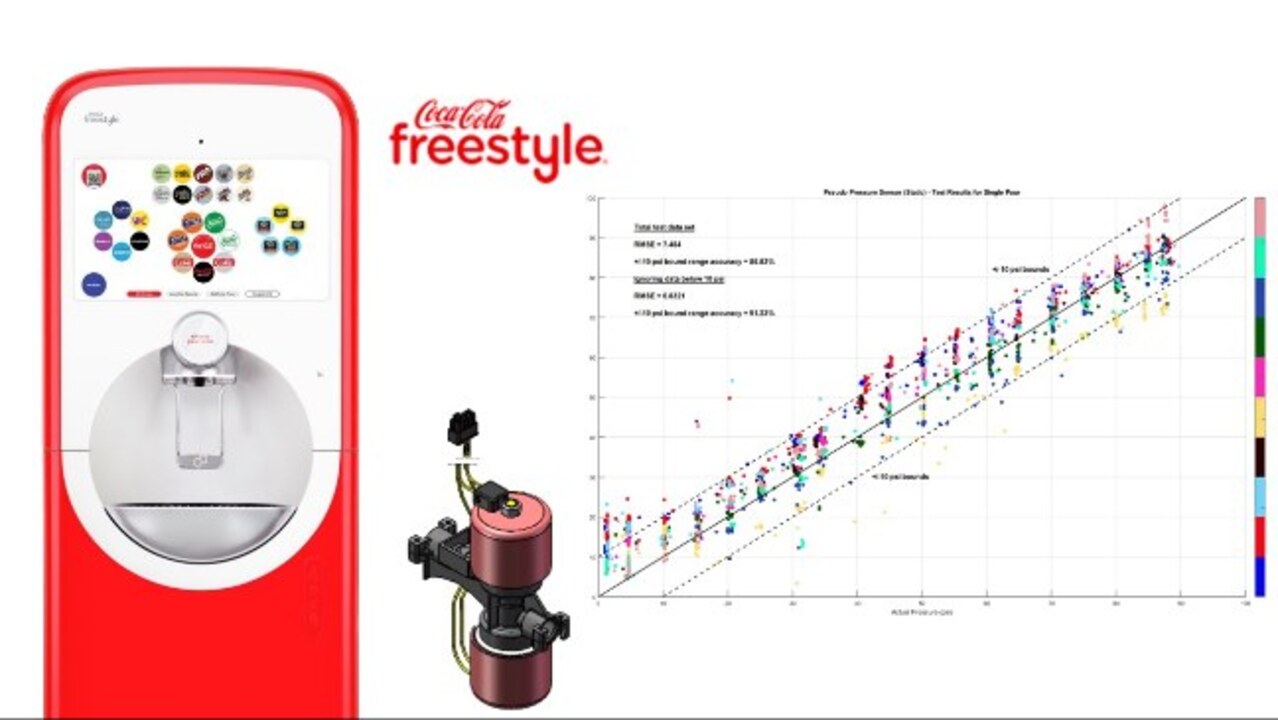
The graph that you see on the screen is from those lab-testing data. Again, it is in the confusion-matrix style. The x-axis is your actual pressure, and the y-axis is the predicted pressure. And we did a lot, of course. We did-- we automated this test. And we did, like, 3,000 tests. And we varied the pressure, again, all the way from 0 to-- you see 90 psi here, but we did up to 140 psi. And that's the graph-- that's the result that you see.
One thing that I want to point out to you guys is that it's-- if you have an actual physical pressure sensor, you're going to get a lot more accurate data. I will concede that, all right. So you probably have data that's perfectly lining up on that diagonal line. But this is a pseudo sensor. And we are getting data that is bound by plus or minus 10 psi.
By that what I mean is that if your actual pressure is 50 PSI, your algorithm might predict it between 60 and 40 PSI. But that is good enough for us. Currently, we have no way of knowing what the pressure-- what is the back pressure against which our valves are opening. But with this pseudo sensor in place, deployed in our dispensers, we know an idea of what that starting pressure is. And that is all we need.
We don't need the perfect data. We want to know whether we are opening against 50 PSI, or we're opening against 10 psi. That is what we are interested in. And this pseudo sensor fulfills that and gives us that idea of what the pressure-- what the starting pressure for our valve is.
So let me conclude by saying that we have developed the pseudo sensor. So this pseudo sensor developed in all three stages. One was a lot of data collection at dispenser condition. Once we collected the data, we had to go do a machine-learning algorithm. Here in this case, it's a linear-regression fit, where we came up with this algorithm that will tell us what the starting pressure is based on the current feedback. And then this algorithm is deployed in our dispensers.
What is this-- what does this pseudo sensor done for us? This is a software pseudo sensor. It is easy to deploy on all our dispensers. It is not a physical pressure sensor. It is in lieu of a physical pressure sensor. And it has significantly transformed our FCM. It is transformed our FCM into a "Smart Component."
What do I mean by that? This FCM, or Flow Control Module, was meant to be a valve for regulating flow rate. That was it's job. It has to maintain a constant flow rate. And that is what-- it has a binary and proportional valve. And the main job of the FCM was to regulate water flow rate.
But now, with this addition of this pseudo sensor, it can also-- this simple Flow Control Module can also tell you the pressure against which the valve started. It can give you the starting pressure. So it has transformed from a simple component to a Smart Component. And it is telling you the environment in which it is operating, the environmental data that it's giving you is the pressure against which it is operating.
And this pseudo sensor has enabled us to do effective diagnostics. Without this pseudo sensor, we cannot do effective diagnostics. We cannot tell you whether it's an FCM problem or if it's a problem before the FCM. So this gives us a data which we originally did not have. And the FCM is giving us the starting pressure data.
This is not a fully complete project yet. It is still an ongoing project. We have deployed these pseudo sensors in the field. We are now in the process of collecting field data. We want to study, what is the field variation of that platform-to-platform variation? Is there variation from dispenser location? How is it looking in Georgia? Maybe it's different in California. Maybe there is a difference between day and night. Maybe there is difference between old FCM and a new FCM.
So we are looking, analyzing all this data. And we want to-- the next step will be how to use this data to do effective diagnostics. That is probably a presentation by itself-- looking at this data and coming up with a diagnostic strategy. So I will leave it for a different day and different occasion. So I will conclude here. So this pseudo sensor has been developed and deployed in our dispenser. And it is so far working well for us. It is giving us data which we did not have before.
Before I conclude, let me also have some acknowledgment here. This is not a one-man job. I get to stand and present, but this is-- a lot of people here at Coke were involved in this work, so a big shout-out to Keith, Jose, Matt, Bin, Hitesh.
And we had a great partnership with MathWorks in doing this work. So they did bring in a lot of skills with that, complementary skills to what we did not have, so a shout-out to Sudheer, Nick, and Roger.
Thank you. I will conclude my presentation here and open the floor for questions. Thank you.
[AUDIO LOGO]
Related Products
Learn More
Featured Product
MATLAB
Up Next:

Related Videos:


Seleccione un país/idioma
Seleccione un país/idioma para obtener contenido traducido, si está disponible, y ver eventos y ofertas de productos y servicios locales. Según su ubicación geográfica, recomendamos que seleccione: United States.
También puede seleccionar uno de estos países/idiomas:
América
- América Latina (Español)
- Canada (English)
- United States (English)
Europa
- Belgium (English)
- Denmark (English)
- Deutschland (Deutsch)
- España (Español)
- Finland (English)
- France (Français)
- Ireland (English)
- Italia (Italiano)
- Luxembourg (English)
- Netherlands (English)
- Norway (English)
- Österreich (Deutsch)
- Portugal (English)
- Sweden (English)
- Switzerland
- United Kingdom (English)