Design Reduced Order Models (ROMs) For Oilfield Processes in MATLAB | MathWorks Energy Conference 2022
From the series: MathWorks Energy Conference 2022
Mayank Tyagi, Lousiana State University
Derek Stall , Cortec
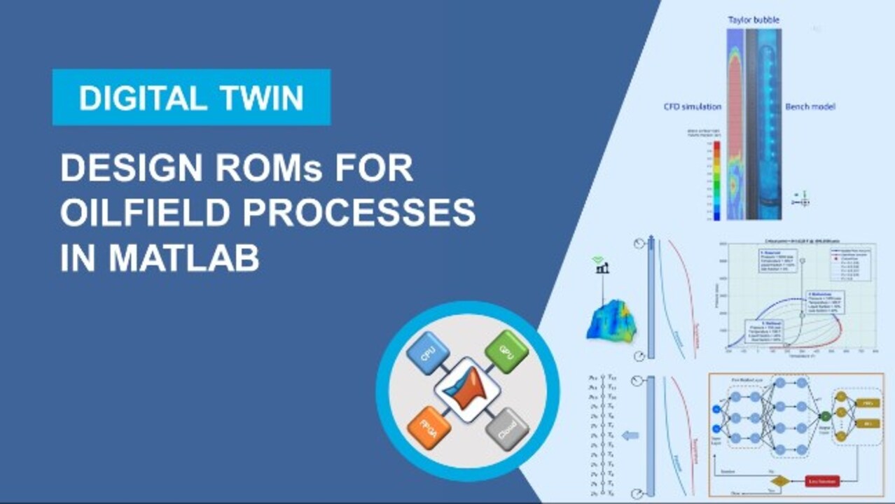
Design a reduced order model (ROM) for oilfield processes to execute computational fluid dynamics (CFD) across wellbores, pipelines, and risers. In this example, the process follows a data-driven modeling approach to simulate multiphase systems with high accuracy using physics-informed neural networks (PINNs) validated and verified against an equivalent laboratory model.
Published: 22 Mar 2023
Hello, everyone. I'm Mayank Tyagi from Louisiana State University. And I'm going to be talking about our research effort in building digital twins of all oil and gas wellbores. This is a collaborative work based upon the graduate thesis of Mr. Derek Staal, who works for CORTEC, and then I'm collaborating with Dr. Oscar Molina from the MathWorks.
Hello.
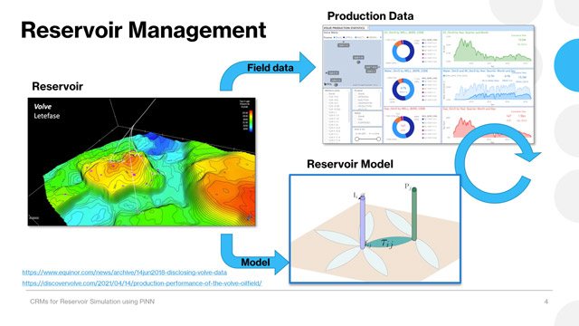
So before we get into the digital twins of specifically for the wellbores, let me give you a lay of the land, which we call the digital oilfield. Digital oilfield, let's start from the lower left corners of the reservoir, which shows all the kinds of assets different wells representation of these subsurface environments you have to use information from the seismic information, the different reservoir characterizations, well logs, fluid properties, and all that.
When you are connected to these wells, throughout their production life, you'll be looking for the well maintenance data. They're monitoring these wells. And all the information that you have from the wells that gets transferred into the central processing facilities, basically, all the oil, water, gas, that you're producing needs to be transported there using flow lines, pipelines, and in issues associated with the pipelines with either flow assurance, optimizations, and then you're trying to look for some event-based monitoring that could be if there are any leak or not things like that.
And towards the central processing unit, you will have a variety of issues like predictive maintenance, or process optimization, and then you're also looking at some economics data when you are putting them into the sales lines. And some of the fluids that you have to send it to treatment, like gas and water. They have their own issues.
One of the things that is very prominent over here, are the type of the data format and the way we are restoring the data at different stages could be quite different. And to take all this information from a variety of distributed data sources, with such a variety, the underlying technology of cloud computing whether the cloud is coming from the AWS issue or some sort of a Google Cloud or for that matter Matlab, these are becoming like an enabling technologies for supporting this idea of digital oilfield.
Specifically speaking, about digital twins, as we mentioned about wells and pipelines, wells and pipelines are the assets that can connect your digital subsurface world to the surface facilities. And therefore, it is very important to actually prepare a digital twin for these wellbores if you wanted to complete the digitization of the entire digital oil field. And to highlight, I'm showing you a CFD animations right next to a wellbore showing you the multiphase-well dynamics that values of simulation can get.
So this is the outline of the talk. We're going to be talking about what is digital twin. Why is variable dynamics so important, and how do we make use of physics-based and data-driven models. And what is the role of big data and IoT for such digital trends in the wellbores? And then we'll have some conclusions.
So in order to kind of define a digital twin, let me take your focus to the right side of the slides. There is a recent review paper in IEEE Access by Gosine et al. which is looking at digital twins of oil and gas industries. But the main focus of it is to define the physical space and a virtual space.
In virtual space, a lot of the people that have been doing simulation, sort of have a misnomer about simulation being a digital twin. But you have to realize a digital twin lies in a space of convergence of physical space and a virtual space. Not only it is taking the sensors' data that are fed into the simulation, but your simulation should be able to send a decision that in the form of a actuator or does something in the physical space. That really is what makes it digital twin.
And to give focus to the big data issues in the oil and gas industries, there is another review paper by Nguyen, Gosine, and Warrian. It is talking about variety of sensors in the oil field. They could be locally stored. They could be in the data center to perform a variety of analysis.
And to achieve the actuations using engines, alarms, or walls they have to rely on some sort of a big-data processing unit, which in our case, is the enabling cloud technology. And in this particular work, we will show the actuations using the flow-control walls for our physical setups that we are making in this particular problem. So over to Oscar.
Thank you, Dr. Tyagi. It is important, as you mentioned, Dr. Tyagi, to make that distinction, or at least to have a clear common ground definition of what is a digital twin. And I'm going to borrow some of the words from my manager, Jonathan Sage.
We had some of these deep conversations sometimes, and then he helped me in defining what is a digital twin as an updated representation of a real asset. I think the key words right here, are the two at the bottom, which is "in operation."
So as you mentioned, Dr. Tyagi, a simulation model does not necessarily mean a digital twin. But a simulation model can actually be part of a digital twin and in fact, can be the most important part of it, but it has to be integrated with real time, not real-time data necessarily, but operational data so that the simulation can actually mimic what is happening in real time.
And digital twins are actually based on a workflow. So we have the workflow that the first stage is to build a digital twin based on a physics-based model or biological models. Or we can actually use hybrid models, for that matter. Then we can leverage the digital twin, which we just built, so we can do predictive maintenance with that model, we can forecast production if it's a rational model, for example, or we can run some type of optimization. And then we deployed it.
And this is where the part becomes very important because if we have digital tools that are using real-time data, the data is the historical data files of the historians, so databases can grow very quickly so that we need the computing power from cloud computing in order to be able to ingest the data and do all sorts of analysis with that data in order to fit back to the real model and just make sure that the digital twin, as a whole, is straightforward representation of the real physical process.
So in this presentation, we are going to talk about how to build a digital twin for a wellbore. So what does that entail? And then we will talk about how to deploy social normally. For now, let me just give you a couple more definitions about the digital twin workflow.
The first one is the hardware twin. So when we have a, take for example, a finite element model of an actual physical device, that's what we call hardware twin. You can run simulations on that FEM model and get simulation results and make design decisions based on those type of modeling approaches.
On the other hand, you also have a software twin. So if you think about the logic of a system, now we're looking at a control system. So it is highly based on logical workflows. So we have decision spaces, and we have logical operations. So that's what we call a software twin.
And we can actually produce really good simulations using these two approaches. But again, we are still lacking the historical or like data in order to make this workflow a reality twin. So as the figure shows here, reconciling these reports putting them all together is what we call building an actual digital tool.
So what does it look like for a world? And why is it important to take into account wellbore dynamics when we are talking about the digital oil field? Well, for once, whatever connects the reservoir with the surface. There's no denying about it. That's the only way we can get the fluids from deep down in the subsurface up to the surface.
And there are many processes that happen right here when we are producing these fluids. So for once, we have the temperature and pressure changes on the wellbore that might not be non-negligible. So they might be significant. And in fact, and over here, I'm showing you the approximate temperature gradient average, so it can grow quite significantly, especially for ones they go way into the surface, right?
So as pressure and temperature changes along the wellbore, so there are some changes in the fluid properties that will affect the performance of a well. I'm going to talk about that on the next slide. So just from this slide, just keep in mind that those pressure and temperature changes happen simultaneously with fluid flow. So this is a highly coupled problem that we are talking about here, OK. But that's the problem that we got to solve in order to connect the subsurface with the surface, OK.
So now, the question is, how can we effectively do this. And let's not forget that if this is to be a digital twin, so we have to reconcile this model with some sort of operational data. So that's the challenge. How can we make this more effectively?
So one of the things that we have been working on is on the fluid properties piece of the model. So we are working on a multi-component analysis with Matlab. So oil and gas, we tend to think about oil and gas as fully defined places, like oil is a liquid phase, gas is a vapor phase, and water is liquid phase as well.
But in reality, oil and gas are made up of a number of components that are in equilibrium with one another. So that dependency of three properties will tied up to pressure and temperature changes in the wellbore and that we can determine those properties, or changes in properties, using vapor-liquid equilibrium calculations.
So you can see right now, that the problem is becoming more and more complex the more we talk about it, right? And of course, now, when we take the fluids from the bottom up, there will be changes that will be felt at the surface, especially when we flash or when liquid flushes into the vapor phase. So we start looking at highly valuable liquids to the gas phase, which might not be as available. So those are changes or considerations that we need to take into account with modeling fluid properties in such type systems.
Here's an example. This is a very simple example in which I want to illustrate how the fluid properties or in this case fluid fractions, liquid and paper fractions, change from the reservoir all the way up to the surface. So right here, the reservoir surface represented at this one circle with the number one here to the left on bottom left, then we have the bottom hole and number two, and then we have the surface of number three.
So in this example, the well starts at this pressure and temperature conditions, right? And typically, with typical reservoirs, you don't lose as much temperature. So you can safely assume that temperature is constant until you hit the wellbore. There might be some changes in temperature in the near wellbore region, but let's just assume that temperature stays constant. All that change was pressure.
But right at this moment, if we look at this envelope, which, by the way, this envelope tells you whatever is above this blue line, which is called the bubble-point line, with the bubble-point curve, whatever is up in this region, is in liquid phase. Whatever is to the right of this red dot, which is called the critical point, is supercritical fluid. And whatever is below it, below this red line, is in vapor phase. And everything else inside of this envelope is in two frames, OK, in two phrases.
So in this example, when we lowered the pressure to this point, so we hit this line right here. So we refer to it in this table. We see that it is at 30% vapor that we have right here as our fluid quantity at that point.
And then, from the world where we've got to flow up to the surface and then more changes happen and then you ended up dropping your pressure up to this point, and now, right here, you have 60% of your fluid in molar water fraction, it's in the vapor place. So a substantial change occurred from this point down to this point. That's why water dynamics matter, OK.
So what we do with typical physics-based models is that we solve the conservation laws of mass momentum energy. And energy, similar to our reservoir simulation but this is for the flow pipes, and there are many variables involved with this set of equations you can see. And then integrating those equations out on the pipe, that might not be vertical, but it could have some changes and deviations and so forth might not be straightforward.
So what you have to do or what is typically done is that you discretize your pipe into different segments, And then you would solve for both pressure and temperature simultaneously in order to get those profiles that you see here to the right side of the slide.
So this is typically done by commercial software. Although, most commercial software assumes steady-state conditions, which might not be suitable for a digital twin. Remember, that the digital twin considers data coming from the operations. Operational data, be it real-time data or near real-time data, in order to reflect the reality of the physics or the physics of the model with the digital twin.
So we need to take into account the trends in terms of the study time terms in these equations. And furthermore, traditionally, we have been using correlations that were built for pressure losses and frictional friction factors for multiphase friction factors and liquid holdups and among other variables, those correlations were based on lab experiments for the definite setups that might not apply to every well. So we also need to be cognizant of those limitations of physics space modeling. And I'm going to turn it back to you, Dr. Tyagi.
All right, thank you, Oscar. So let me kind of rush through on how we actually created that physical setup. So this work is based on Derek Staal's master's thesis work. There are edge devices on Raspberry Pi as well as Arduino. And the actual setup is trying to do a slug flow control, which is a specific flow regime that is intermittent.
And the pressure signal that is obtained through the pressure transducer at the bottom of the riser is used as the diagnostic where if we could actually eliminate the oscillations in the bottom hole of the riser, we are able to achieve that flow control problem.
So this is a flow control problem, specifically for our deep water operations and production operations where we can actually see this type of transient, intermittent, pressure oscillations. And to enable all this data transfer, we are going to be using the Azure platform for the cloud computing.
Not only we built up a small bench scale setup, but we also built up like a 28-foot riser model. This is to show another physical setup that tells that the data, the delay, the latency, and the difficulty of achieving this kind of a flow control. There is a huge impact of the length scales of this particular problem in achieving the kind of control that you are trying to get.
And the reason I'm trying to show this at the PERTT lab, is there is also a fully instrumented well with a depth of nearly 5,000 feet deep with fully instrumented and fiber optic that is available at LSU's PERTT lab. So the first step, this was a physical setup. We are trying to show through a simulation model, how do we actually get this intermittent, multiphase, flow patterns.
So for that, we are going to use a volume of fluid model. We performed the great independence test. We did perform the validation for the Taylor bubble lines as well as bubble-rise velocities. And then we demonstrated, using the PID controllers, how do we suppress the flow in bottom hole pressures. This work was presented in the couple of IMECE papers by our team.
So here are some simple CFD results that is showing how the Taylor bubble is formed. The shape of the Taylor bubble is in the form of a bullet-nosed bubble. On the rightmost part, we are able to show that the length of the Taylor bubble predicted by the CFD simulations matched perfectly with your-- very accurately, actually, with the bench scale model. And similar results were obtained from the valor scale star. And then including the Taylor bubble riser, velocities were predicted accurately.
So now that we have validated the simulation model against the physics-based model, the tie-up comes up is in the actuation part. How do we actually come up with a PID controller and transfer that information using the cloud technology?
And for that, we are trying to extend this work also in the area of physics-informed neural networks using the long short-term memory networks. On the right hand side, I'm showing you from Colah's Blog a structure of our recurrent neural network, which is a sequential network that has a unit which we call LSTM unit, comprising of input, output, and forget gate.
There is always a hidden cell states. And then though there are several alternatives available for two LSTMs, but we have transformers and GIUs. We are going to be sticking to LSTMs and try to get the forecasting of these variable behaviors. We will look it into simpler models that have better explainability and interpretability. The interpretability here is trying to establish a cause and effect so that these types of data-driven models are not completely treated as a black box.
So that brings us back to the part where Oscar was mentioning about the governing equations of the unsteady fluid-flow. We use this unsteady governing flow of governing equations as the constraints in our neural networks.
So there is a new paradigm for enforcing the physics into these neural networks. It's called physics-informed neural networks, where your inputs, in this particular case, could be the flow rates of different phases and different sections where we are measuring the pressure drops. We can use that information from the wellbore to train our models, and then, once we make the predictions, and we find an error, we correct for that in terms of making the pressure losses more accurate.
But then we don't just stop at that. We try to use all the physical variables that are in the governing equations to take the regression and then try to satisfy the PDs and the boundary conditions as a part of our problem. And this actually will next include all the vapor liquid calculations as well as multiphase friction pressure drops, including the hold-up information instead of prescribing them to some sort of a correlation.
To that end, if I were to summarize our work. We have been able to demonstrate that to connect the wellhead operations at the surface to the digital representation of the surface it is imperative that we must build the digital twins of wellbores. Without that, it's just not going to be able to give realization to the digital oilfield.
We demonstrated, through two physical models, one advanced scale, which is around three-feet riser and then around the pilot scale model, which is 28-foot riser, that we could achieve the multiphase flow control through physics space through devices that have IoT Edge devices. And we were able to transfer that data to cloud computing. We had validated the simulations.
And we also are encouraging people to kind of invest into our research at the LSU PERTT lab, which is actually a 5,000-foot fully instrumented fiber optics to build digital twins for wellbores in the field-scales. One of the crucial future work that is coming up is physics-informed neural network that can use real-time field data.
And it will be using highly resolved multiphase simulations, and then it will address the technological gaps in the wellbore and pipeline models for multiphase flow assurance. Particularly, it will take us away further from the empirical models based upon the fluid properties as well as friction factors that are not directly applicable to the case that we are solving for.
With that, I would leave the question and answers. And these were the most relevant references for our work. Two of the papers that were presented at the IMECE conference Derek Stall's master's thesis and using the IoT Edge computing device through Cloud by Jensen.
Thank you for your attention, and we are ready for questions.
Thank you very much.
Related Products
Learn More


Seleccione un país/idioma
Seleccione un país/idioma para obtener contenido traducido, si está disponible, y ver eventos y ofertas de productos y servicios locales. Según su ubicación geográfica, recomendamos que seleccione: United States.
También puede seleccionar uno de estos países/idiomas:
América
- América Latina (Español)
- Canada (English)
- United States (English)
Europa
- Belgium (English)
- Denmark (English)
- Deutschland (Deutsch)
- España (Español)
- Finland (English)
- France (Français)
- Ireland (English)
- Italia (Italiano)
- Luxembourg (English)
- Netherlands (English)
- Norway (English)
- Österreich (Deutsch)
- Portugal (English)
- Sweden (English)
- Switzerland
- United Kingdom (English)