Three Steps to Simulate RF Transceivers in MATLAB
Learn three simple steps to design RF transceivers, integrate them in your existing MATLAB code, and perform system-level simulation. With this new approach you can directly integrate RF models in MATLAB for the simulation of digital communication (5G, WLAN, etc.) or radar systems.
Practical examples will demonstrate how to perform RF budget analysis and estimate the impact of S-parameters, non-linearity, and noise. You will see how to customize your RF model to include effects such as impedance mismatches, saturation, and finite isolation.
You can add analog / digital data converters and control logic to the RF transceiver and develop innovative architectures. With this new methodology, you can simulate the entire system in MATLAB together with digital signal processing algorithms. Finally, you will learn how to use multi-carrier Circuit Envelope simulation for coexistence and interferer analysis.
Highlights
- Designing RF transceivers at the system-level
- Using S-parameter, noise, and non-linearity data for RF budget analysis
- Integrating RF system simulation in your MATLAB code
- Using multi-carrier simulation for coexistence and interferer analysis
About the Presenter
Dr. Giorgia Zucchelli is the product marketing manager for RF and mixed-signal at MathWorks. Before joining MathWorks in 2009 as an application engineer focusing on signal processing and communications systems with specialization in analog simulation, Giorgia worked for two years at NXP Semiconductors on mixed-signal verification methodologies. Before then, she worked for Philips Research, where she contributed to the development of system-level models for innovative telecommunication systems. Giorgia has a master’s degree in electronic engineering and a doctorate in electronic engineering for telecommunications from the University of Bologna. Her thesis dealt with modeling high-frequency RF devices.
Recorded: 30 Apr 2021
Hello, and welcome to this MathWorks presentation on RF transceiver design and simulation using MATLAB. My name is Giorgia Zucchelli and I am the Technical Marketing Manager for the RF and Mixed Signal Product areas here at MathWorks. I joined MathWorks in 2009 as an Application Engineer here in the Eindhoven office. In 2013 I transitioned to my current role where I'm currently responsible for the RF, Antenna, and Mixed Signal products. You see here on the slide my email address. If you have any questions related to this presentation, or maybe to the topics of RF and Mixed Signal, please don't hesitate to reach out directly to me.
In the next half hour, using code examples and executable models, we will describe in three simple steps first, how to use MATLAB for the design of RF transceivers starting from high level specifications. Then we will show how to elaborate the RF models to include impairment, or maybe to describe RF architectures in more details. And finally, we will show how to combine accurate RF system-level simulation with digital signal processing in MATLAB.
The motivation for the workflow that I would describe is really simple. We want to directly connect with the power of MATLAB for digital signal processing with RF system-level simulation. Many wireless and radar system designers use MATLAB for the development of complex baseband signal processing algorithms. However the move towards higher frequencies in the millimeter wave range, larger bandwidth, the additional challenges of coexistence are creating an additional complexity for which the RF transceiver's behavior needs to be taken into account in the system design. This is not any more optional. It is necessary. For this reason simplifying the RF model based on simple mathematical expressions is often not good enough. To enable system design we need a better approach to include RF effects directly into your model system simulation. But before we enter into the specific workload details, let's look at a simple example.
This MATLAB script generates a standard compliant 5G waveform and measures the EVM according to the 3GPP standard. The script is based on an example that comes with 5G toolbox. In the documentation you can find many examples that can be used to generate and analyze 5G signals. Additionally, you can perform physical layer simulation, as shown here. In the script we first set up the simulation parameters. In this case, we use the new radio reference channel FR1 with 100 megahertz bandwidth and 30 kilohertz subcarrier spacing. With a single command we generate the reference waveform. The variable txWaveform is a complex array with more than one million samples, and a time duration of 10 milliseconds.
In this example, we perform a common task for the simulation of the physical layer. We're streaming the 5G signal through a simplified RF model. In this case, the model is a simple polynomial expression that captures the gain and third order non-linearity of the transmitter. You're probably familiar with the complexity and the limitations of describing another system using this approach. This is far from sufficient to fulfill the modeling needs of modern RF systems. Although you can create more complex mathematical models, they are hard to maintain and share.
Here we compare the spectrums of the input and resulting output signals. We immediately notice a problem with the simulation, and namely that the simulation bandwidth is not sufficiently large to capture the spectral regrowth caused by the third order non-linearity. We need to increase the simulation bandwidth. This is done by making use of an interpolation filter. In this modified version of the script we use the power of MATLAB to design an FIR multirate filter with a single function call. We interpolate the signal with an oversampling factor of five. Now with the complex array the xWaveform has more than six million samples, and a turn stat at least 5 times smaller than before.
We now stream the interpolated signal through our simplified RF model, and we can view the results on the spectrum analyzer once again. Notice that now we can see the impact of the spectral regrowth due to the third order non-linearity. We're now ready to measure the signal AVM. But before that we need to decimate the signal and perform signal recovery. The EVM of the signal is computed and the result is plotted as a function of the signal slots. As you can see the RMS AVM is approximately 1% and the peak AVM is approximately 4%. Let's now modify this script to include a more refined model of the RF transmitter.
Using the RF Budget Analyzer app we implement a simple transmitter array map with a modulator, a filter, and an amplifier. For each of the components we can provide the specifications and we can inspect the resulting gain, power, OIP3, and noise budget. You can see here, the overall gain is 20 dB, the output OIP3 is approximately 10 dBm, and the noise figure approximately 11 dB. Although this is a simple example, you can see the RF Budget Analyzer allows you to model more complex systems. For example RF systems that make use of S-parameters data. And for example using direct conversion architectures. Recently harmonic balance has been added, and this facilitates more accurate analysis of nonlinear systems such as RF transmitters.
Now that we have analyzed the RF budget of the transmitter, we can export to MATLAB and create an object that can be directly used in the MATLAB script to increase the fidelity of the physical layer simulation. We first need to change the sample time of the RF transmitter object to be consistent with the sample time of the sample 5G waveform. Then, we can stream the upsampled 5G waveform through our RF transmitter object. Once the simulation is finished we can view the resulting spectrum. We see the effects of the non-linearity, along with increased noise floor. We now measure the EVM. As a result of the additional filtering, noise, and cascaded non-linearity, the EVM performance has been significantly impacted and subsequently degraded.
Let's now discuss, what is the underlying technology behind these RF system object, how it was created, and how it can be extended to model even more sophisticated RF systems. Let's recap now how to design transceivers in MATLAB. The RF Budget Analyzer app is an excellent starting point for the design of RF transceivers. With the app you can perform the cascaded analysis of your transmitter over your receiver. You can compute the noise figures, power levels, while accounting for the component's linear, nonlinear noise behavior, along with impedance mismatches between the components inside the cascade. And this is not easily done when using, for example, a spreadsheet or idealized link budget formulas.
The RF Budget Analyzer app has been recently enhanced also to include the harmonic balance. From the app you can generate MATLAB scripts for design space explorations. You can also export automatically generated models for circuit envelope simulation. We have seen how the app can be used to develop a simple line up. But it can also be used to develop more complex architectures. And it is particularly helpful when you want to see the impact of S-parameters data on the overall system performance.
Today, however, we focus on the export capabilities of the RF Budget Analyzer app. There are different export workflows, and each workflow targets a different use case. You can export the RF Budget object to the MATLAB workspace. This is useful, for example, if you want to save the results of one or many analyses, or share the results with colleagues. You can also create a MATLAB script to automate the RF Budget Analysis over multiple corners, or if you want to explore a large set of design parameters. And last but not least, you can export to RF blocks and models and test benches that use the circuit envelope simulations.
Today we focus on the first export option, the creation of another budget object in the MATLAB workspace. Once the object has been exported we can visualize the budget. And from it we can create an RF system that can be directly used in MATLAB. Notice that the RF system object is not an RF Budget object. It is not a static analysis tool. On the contrary, it specifies the sample time, and the center frequencies of the input and output signals. And this makes it suitable for directly streaming into MATLAB. Let's see this step in practice.
From the RF Budget app we exported the Budget object to the MATLAB workspace. We can inspect its properties and the budget results. By default, the object is called RFB. From the RF Budget object we can create an RF system object. We can set, for example, a simple time to be one microsecond. To create a simple signal to test our RF system, we first create a timed vector with 1,000 samples, and the sample time, again, of one microsecond. Then we create a simple sine wave with an amplitude of 10 millihertz, and a frequency of 10 kilohertz. We can stream our sine wave through the RF system, and at last we can plot the results. As you can see, the output signal is amplified and compressed due to the non-linearity of the system.
As you could see from the simple example, it's really easy to simulate RF systems in MATLAB. Let's now dive a bit deeper and understand the underlying technology, and how we can elaborate further the simple model that we just created. When working on wireless communications or radar systems, RF models are necessary and beneficial for many reasons. And here I would like to mention a few. First you will use RF system level models to define and design the architecture and specification of the RF components. You will need models to develop adaptive algorithms such as digital predistortion, automatic gain control, or adaptive beamforming. A model will also be helpful to test and debug the implementation of the transceiver before going into the lab. Or, once you are in the lab you can use a model to better understand the results of your measurements. A model is also helpful to gain insights into the design by comparing measurements and simulation results for directly using the measurements results in your simulation model. And last but not least, the model represents a way to exchange the executable specification, for example, with your colleagues or your customers.
However, RF models need to be fast to simulate. And they need to be sufficiently accurate to be useful. If we visualize the trade-off between simulation speed and modeling fidelity, a whole spectrum of simulation techniques can be used. For most RF simulations, using transient is prohibitive, simply because the required time step is too small and the simulation would take too long time. For this reason, many RF system designers use the equivalent baseband approach, where only the RF behavior around the fundamental frequency is simulated. This approach is fast, as the time step is commensurate to the signal bandwidth rather than the signal carrier frequency. However, this approach has also several limitations. For example it's not possible to use this approach to model out-of-band interfering signals, or to model the non-linearity.
The circuit envelope approach extends equivalent baseband by using multiple carrier frequencies. And therefore it provides a balanced trade-off between simulation speed and modeling fidelity. Circuit envelope separately models the signal modulation, or envelope, and a carrier frequency. Commonly the envelope bandwidth and the carrier frequency are different by at least an order of magnitude. This makes circuit envelope faster compared to transient. Harmonic balance analysis is performed at the carrier frequencies, and is used to determine the harmonics in the mixing product. With circuit envelope, an harmonic balanced analysis is executed at every single time step, thus producing a time varying envelope centered around each of the simulation frequency.
Without entering into the details, each input signal is specified to have a unique carrier frequency. The software uses the harmonic balance to compute all the resulting harmonics and modulation products, and then it returns the desired envelopes back for subsequent processing. As you can see this approach is more sophisticated and is more accurate compared to equivalent baseband. But how does circuit envelope and how does this approach related to our RF system object? When we created the RF system object in MATLAB another blockset circuit envelope model was also automatically created. This model actually exists, if you want, behind the scenes, and is used for the circuit envelope simulation. When you invoke the object in MATLAB, the input signals are directly passed to the Simulink input board, streamed through the signal, and the output for signals are returned back as return arguments from the object.
Once we create a data system object, we can open and modify the associated Simulink model. By accessing the Simulink model, we can increase the complexity of the RF system. There are, of course, limitations to the type of modifications that you can make. And it is a rule to remember, is that you should not change or should never touch the input and the output blocks. A simple example of the modifications that you can make is, for example, adding blocks to the Simulink diagram, or changing the parameters. Here for example, we added a spectrum analyzer to visualize the results. And we also added phase noise and LO to RF leakage in the RF modulator. This might be a little bit overwhelming. But the RF blocks that support envelope library has a very rich set of components that you can use to model almost every transmitter and receiver.
You can add linear blocks such as multipurpose parameters, non-linear blocks such as power amplifiers with memory effects, mixer with intermodulation tables, different sources of noise, color noise distribution for example, tunable blocks to model adaptive architectures, and many, many more. And if you cannot find a specific RF component, well that's not a problem because you can use the Simscape modeling language to author your own.
This brings us to the last aspect of the workflow, and the last step. We started from an RF Budget object. We created a model that makes use of circuit envelope. We show how to elaborate this model to add more details. Now we'll talk how to enable the simulation of the system in MATLAB. Using the RF system object in MATLAB is straightforward. The input argument are passed to the input ports of the model, centered around a certain frequency. The output port return the signals and present the return arguments of our object. Beside multicarrier simulation, another benefit of using RF boxset circuit envelope is that impedance mismatches are properly captured. And this is really hard to do when you use spreadsheets or simple mathematical equations to represent your RF system in MATLAB. On top of this, the internal states of the simulation are preserved. So you can execute the RF system and frame by frame and in between invocations-- for example, the states of filters or of S-parameters will not be reset. In other words, the simulation results will be correct.
So far we have seen examples that use a single input and output port But direct conversion architectures are also supported, and they make use of two import ports or to output ports to represent the interface and quadrature components of your systems, I and Q. And last but not least, the Rf system object parameters can also be adjusted to model multiple input signals centered around different frequencies, or multiple output signals centered around different carrier frequencies. This is very convenient, for example, to model the effects of an out-of-band interfering signal. In this first simple example we use the RF Budget Analyzer app to implement a direct conversion receiver, as we can see from the zero Hertz output frequency. In the generated model you will notice that there are two separate I and Q output branches. And when we invoke the RF system object associated with the system, the output signals I and Q represent the real output signals centered around zero Hertz. Port number one will return the enphase argument and port number number will return the quadrature argument.
This other example we usd the RF Budget Analyzer app to describe a low IF receiver. In this case, the local oscillator is centered at 2.45 gigahertz. And IF output signal is centered at 50 megahertz. Let's make, for example, the assumption that we want to analyze the impact of an image signal, and that we want to experiment with an image rejection filter. In this case, with our RF system object, we can just specify to input carrier frequencies. The first carrier frequency will be representative of our input signal at 2.4 gigahertz. The second carrier frequency would be representative of our image signal centered a 2.5 gigahertz. Because 2.45 and 2.5 are equally spaced from the local oscillator centered around 2.45 gigahertz, both our input signal and our image signal will be down converted to 50 megahertz and returned by our RF system object. In this case the input argument of our RF system would be an array with two columns, each representing the modulated waveform centered around each of the input carrier frequencies.
These introductory examples demonstrate the flexibility of the RF system workflow. By directly modifying the associated model and making use of Simulink as a canvas to draw your RF transceiver architecture, you can really explore a wider range of applications and directly test them in MATLAB, for example using or reusing existing MATLAB code. In this diagram, for example, we extended the RF system model to include a power amplifier that is based on real measurements, capturing both non-linearity and memory effects. We included the upconversion stage and impedance loading of the antenna. We also have an observer receiver that monitors the output of the PA, and we use this observer receiver to close the power amplifier in a feedback loop and insert a digital predistortion algorithm for its linear recession.
With this, I would like to conclude. We have seen how to combine the power of MATLAB for signal processing with accurate RF system simulation. You saw how to take advantage of Simulink and circuit envelope simulation offered by RF Blockset, model RF transceivers, and how to integrate this simulation in MATLAB using a straightforward approach. In this way you really have the best of both worlds. And I thank you very much for your attention. I invite you to try MATLAB RF Toolbox, RF Blockset in your next design, and also all the other MathWorks add-ons that can be helpful for the design of wireless communication systems or radar systems.
Well the examples that we covered today are shipping with the product. So if you have, for example, the RF Blockset, you will see all the examples that we covered. If you have questions, please don't hesitate to reach out. Thank you very much.