Tuning and response optimization of extracted coupled-resonator filter models

Welcome to this video which highlights the use of MathWorks products for coupled-resonator model extraction workflows. In today's video, we will be talking about how models extracted for coupled-resonator filter structures can be tuned and optimized using a new MATLAB-based workflow. As stated, we are going to be covering some new techniques relevant to model extraction of coupled-resonator filters. We will cover how this workflow can be implemented in a MATLAB application constructed using App Designer.

New techniques for this workflow include streamlining of the phase, the embedding step of the workflow, along with additional coupling matrix output formats. Finally, an innovation to this workflow is described wherein nodal tuning of the coupling matrix can be performed via lumped element components. Nodal tuning can be combined with a specialized optimization methodology to achieve desired electrical performance, including passband equiripple return loss responses.

This optimization technique can be readily integrated into a RF microwave coupled-resonator prototyping development workflow, as well as directing the mechanical tuning of cavity filter structures. One of the main highlights of the model extraction workflow is how MATLAB can be used as an aid in RF microwave component design. I want to reiterate a few of the key themes that are commonly used for coupled-resonator model extraction.

First, you can make use of MATLAB to access measured or simulated S-parameter data. Second, you can develop algorithms using MATLAB to characterize your RF data. We make use of functionality from MathWorks RF Toolbox to convert S-parameter data into a Laplace domain representation so that a coupling matrix representation of the coupled-resonator filter can be realized.

Finally, this model extraction process could be integrated into both a coupled-resonator prototyping workflow as well as into a mass production environment where thousands or tens of thousands of coupled resonator filters are tuned by trained floor personnel for such things as base station applications. In today's video, we are going to talk about workflow enhancement, which will readily facilitate these previously described themes.

MATLAB can readily interface with vector network analyzers. MathWorks partnerships with major test equipment manufacturers. Common communication protocols supported via MathWorks Instrument Control Toolbox can interface with vector network analyzers. Today, we will be making use of a Keysight Fieldfox microwave analyzer to characterize the electrical behavior of a high-performance dielectric resonator cavity filter. Let's talk about the basic coupled-resonator cavity model extraction workflow.

We begin the workflow by obtaining S-parameter data, usually from a network analyzer, but this data can also be generated via EM or RF analysis software. Now what we need to do is transform the S-parameter data into a format that will allow us to extract a nodal model. In this case, I'm going to convert the S-parameters into Y-parameters and then use a rational fitting technique to extract the Laplace domain model.

The Laplace domain model will have twice the number of poles as the filter has individual resonators. This constraint is necessary to derive a behavioral model that can be directly compared to the golden reference synthesis model. Once the passband Laplace domain model of the Y-parameters has been extracted, it will be necessary to convert it to the lowpass domain. Thus, the derived poles and residues of the passband model will be converted to a lowpass domain equivalent, and the number of poles will be reduced to the same number of poles as the cavity filter.

This allows me to construct the load source transversal coupling matrix that can be converted into a folded format and then subsequently optimized to realize a format that resembles the form of the golden reference coupling matrix. Once the desired coupling matrix format has been obtained and optimized, the network parameters corresponding to this matrix format can be calculated and compared to the measured result. This quantifies how well the optimized coupling matrix structure describes the behavior of the actual cavity filter.

Notable workflow enhancements are going to be covered later in this presentation. This workflow can be used to complement the traditional RF microwave filter design workflow. This workflow can be used to shorten the development time of coupled-resonator filters. This workflow can add value in a manufacturing environment. Particularly, the techniques can be used to either semi or fully automate the cavity filter tuning process. With the new capabilities introduced in today's presentation, a tangible roadmap is laid out showing how each of these goals can be achieved.

In the 2024 release of MATLAB, MathWorks RF PCB Toolbox became home to the coupled-resonator model extraction workflow. On the accompanying slide, you can see that the associated MATLAB function is called measuredFilter, and it has several properties which allow you to determine a coupled-resonator filter's coupling matrix and individual resonator unloaded Q factors. Links to the associated documentation are listed on the slide. I have incorporated this functionality into a MATLAB application which streamlines the model extraction workflow.

Packaging of this workflow into a single MATLAB application permits for a more user-friendly experience. You will notice that there are five panes that constitute the application, and these follow the technical computing workflow. The first pain permits a user to access measured or simulated coupled-resonator filter data, either from a vector network analyzer or through an upload of S-parameter data. You will notice that there are three green push buttons on the first pane. Each of these green push buttons are for working with data from a network analyzer.

The leftmost push button sets up communication between MATLAB and a network analyzer. An appropriate calibration of the network analyzer is recalled from memory so that properly calibrated network parameter measurements are made. The push button to the immediate right of the first push button facilitates a read-in of the network analyzer data into MATLAB. Use of network analyzer specific skipping commands are necessary so that both the S-parameter and frequency data can be properly imported to MATLAB.

The rightmost green push button, Write S-parameter File, is self-explanatory as the imported S-parameter data can be written to an S2P data file through a dialog interface. If you choose to import S-parameter data from a file rather than via network analyzer measurements, you will also notice that once S-parameter data is imported, each of the four S-parameter elements are plotted in a dB magnitude versus frequency format.

In the second pane, one needs to specify some basic properties of the coupled-resonator filter structure. Specifically, one needs to specify the number of resonator elements that populate the filter along with the filter's approximate center frequency and equiripple return lost bandwidth. For the demonstration example, the filter order is 8, the nominal center frequency is 2.115 gigahertz, and the equiripple bandwidth is 10 megahertz. Once these parameters, one can execute the functions that correspond with the Extract Lowpass Admittance Poles and Residues push button. You will notice that a set of admittance poles and residues are calculated and echoed in the application pane.

Recall that the S-parameters are converted into an equivalent Y-parameter format, and that the passband poles and residues are converted into a normalized lowpass domain format. With this set of poles and residues, the filter's transversal coupling matrix can be determined. At this point, the necessary steps for calculating the extracted coupling matrix have been completed. Once the third pane has been selected, you will notice that there are several push buttons for determining different configuration of the coupling matrix.

As previously stated, the transversal coupling matrix can be directly determined from the normalized admittance poles and residues. Once we have the transversal coupling matrix, it can be converted into the folded coupling matrix format by pushing the Perform Canonical Matrix Rotations push button. If the physical realization of the filter is not in folded form, one can make use of the Perform Isospectral Optimization push button. You will need to specify both the optimizer step size as well as the number of iterations for the optimizer to execute.

Typically, a step size of 0.125 and 2,500 iterations provide satisfactory solutions. For isospectral optimization, it is necessary to define a target matrix configuration. A logical matrix can be used to define the desired nonzero coupling matrix elements. Once the coupling matrix is in a desired state, an estimate of the unloaded Q factor for each of resonator structure can be calculated and reported in the rightmost pane. These unloaded Q factors directly correspond with the filter's passband insertion loss.

Obviously, once an extracted model has been identified, it is necessary to validate the model against the data set which was used to create the model. In the fourth pane of the application, a comparison is made between the S-parameter data accessed using the first pane and S-parameter data generated from the extracted coupling matrix model. You can see that there is favorable correlation between the original data set and the S-parameter data generated from the extracted model.

You will also notice that there are additional push button options which go beyond the model validation step. You will see that the lower left-hand push button allows you to write normalized lowpass rational function representations of the ABCD parameters to a MATLAB data file. These ABCD rational function representations can be used for network synthesis analysis. On the right-hand side of the pane, you will notice that you can write a unique representation of the S-parameter to a Touchstone data file. N plus 2 parameter files describe a nodal representation of the coupling matrix topology with each node port, as well as external ports, being terminated with appropriate loads.

In one case, a lossless S-parameter matrix is exported and the other push button option produces a lossy representation. The lossless representation is ideal for use in combination with a customized optimization algorithm that can be used with Chebyshev and generalized Chebyshev filter responses. At this point, a new element to this workflow is introduced which can be used to complement the coupled-resonator development workflow.

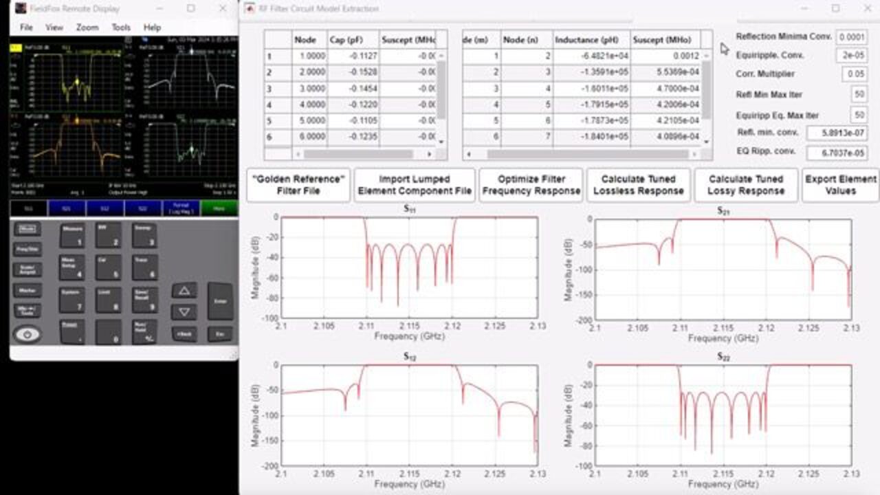
In the final pane, the nodal matrix representation of the measured data can be tuned to achieve a desired electrical performance. From the previous pane, both the lossless and lossy n plus 2 S-parameter matrices were automatically generated. You can see that in the top half of the pane, there is a listing of shunt capacitor and inductor elements where you can either populate the table elements or import values from a MATLAB data file. And these are then used to tune the filter response.

You will notice that for S-band responses, you would typically specify capacitor values on the order of sub-picofarads and inductor elements on the order of microhenries. A golden reference filter file is required for the optimization process as this file contains the reflection zeros which are used in the optimization process. Once the golden reference filter file and an initial set of lumped element component values have been selected, there are several user-specified optimization settings that need to be supplied for the optimization process.

This includes specification of the convergence for the reflection zero diagonal element values, the standard deviation of the local maxima of the passband return loss response, the number of iterations used for reflection zero convergence, along with local maxima standard deviation convergence. Finally, one can also specify the correction vector multiplication factor. This value should be between 0 and 1, and typically, one would set this between 0.025 and 0.25. This parameter is a contraction factor of the correction vector calculated via multivariate Newton-Raphson root calculation.

Once the optimization algorithm has achieved the desired level of convergence, you can plot both the lossless and lossy responses of the optimized network. You will notice the near ideal equiripple return loss characteristics produced via the optimization technique and the updated element values calculated. These lumped element values can be subsequently mapped to coupled-resonator tuning elements such as resonator and coupling screw insertion depths.

Use of this tuning optimization methodology yields filter responses that correlate with golden reference filter responses which are obtained during the software design stage of the RF microwave filter development process. Inclusion of such techniques can potentially have a substantive impact on the duration of the coupled-resonator filter design and development process. Although not detailed during the demonstration of the MATLAB application, the technique used for filter port de-embedding has been recently improved. Use of an excess number of poles to fit the diagonal elements leads to an accurate estimate of the phase offset at each filter port.

For instance, if an ideal filter has eight resonant sections, the number of rational fitting poles required would be 16. When there is an extra section of transmission line at each respective filter port, the diagonal elements require more than 16 poles for appropriate model extraction. Typically, these excess poles are characterized by a real axis pole that is multiple orders of magnitude larger than the filter center frequency and then as many as two complex conjugate pole pairs where the imaginary pole frequency is noticeably larger than the filter center frequency.

The de-embedded phase can be determined using these excess poles, and then these phase offsets can be de-embedded from the S-parameter data to obtain a rational fit with the appropriate number of poles. A substantive extension to the coupled-resonator model extraction workflow is that now the extracted coupling matrix can also be represented by an N plus 2 S-parameter matrix.

The N plus 2 S-parameter matrix can be tuned with lumped element components, and tuning of the filter can be achieved via optimization. In this case, simultaneous optimization of the diagonal element electrical performance at the reflection zero frequencies of the filter, along with dynamic adjustment of the reflection zero frequency values, render a filter performance with an equiripple return loss response column.

So to wrap up this presentation, let's review a few of the key things that were discussed. An updated version of the coupled-resonator model extraction workflow was presented. Portions of the workflow can be executed with the function measured filter, which comes with MathWorks RF PCB Toolbox. The implementation of the workflow is application based, wherein the RF PCB Toolbox function measured filter is principally used.

Several new differentiating elements are available in this workflow to improve aspects of the analysis, the user experience, as well as widening its applicability in the coupled-resonator filter development workflow. Thank you for watching this video. And I would encourage you to try this new function, which is available in MathWorks RF PCB Toolbox, and to contact MathWorks if you have questions about the technical updates in this workflow.