vggishEmbeddings
Description
embeddings = vggishEmbeddings(audioIn,fs)audioIn
with sample rate fs. Columns of the input are treated as individual
channels.
embeddings = vggishEmbeddings(audioIn,fs,Name=Value)embeddings =
vggishEmbeddings(audioIn,fs,ApplyPCA=true) applies a principal component
analysis (PCA) transformation to the audio embeddings.
This function requires both Audio Toolbox™ and Deep Learning Toolbox™.
Examples
Download and unzip the Audio Toolbox™ model for VGGish.
Type vggishEmbeddings at the command line. If the Audio Toolbox model for VGGish is not installed, then the function provides a link to the location of the network weights. To download the model, click the link. Unzip the file to a location on the MATLAB® path.
Alternatively, execute the following commands to download and unzip the VGGish model to your temporary directory.
downloadFolder = fullfile(tempdir,"VGGishDownload"); loc = websave(downloadFolder,"https://ssd.mathworks.com/supportfiles/audio/vggish.zip"); VGGishLocation = tempdir; unzip(loc,VGGishLocation) addpath(fullfile(VGGishLocation,"vggish"))
Read in an audio file.
[audioIn,fs] = audioread("MainStreetOne-16-16-mono-12secs.wav");Call the vggishEmbeddings function with the audio and sample rate to extract VGGish feature embeddings from the audio. Using the vggishEmbeddings function requires installing the pretrained VGGish network. If the network is not installed, the function provides a link to download the pretrained model.
embeddings = vggishEmbeddings(audioIn,fs);
The vggishEmbeddings function returns a matrix of 128-element feature vectors over time.
[numHops,numElementsPerHop,numChannels] = size(embeddings)
numHops = 23
numElementsPerHop = 128
numChannels = 1
Create a 10-second pink noise signal and then extract VGGish embeddings. The vggishEmbeddings function extracts feature embeddings from mel spectrograms with 50% overlap. Using the vggishEmbeddings function requires installing the pretrained VGGish network. If the network is not installed, the function provides a link to download the pretrained model.
fs = 16e3;
dur = 10;
audioIn = pinknoise(dur*fs,1,"single");
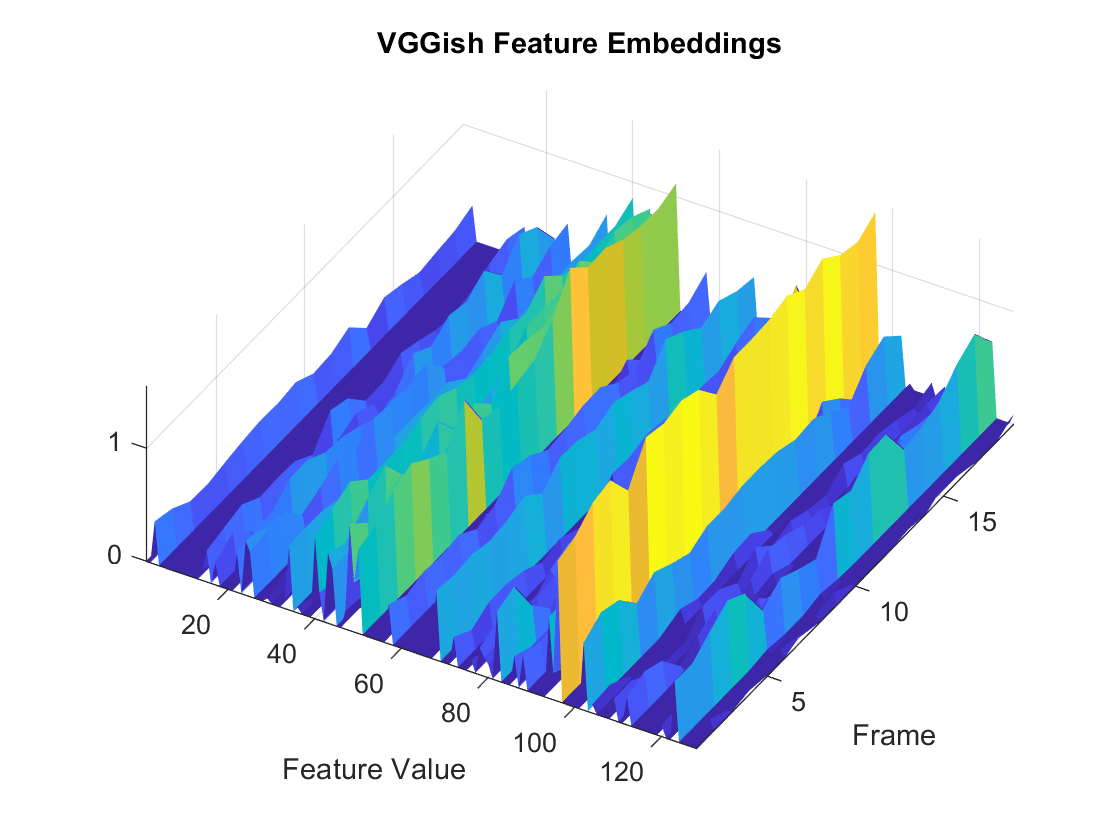
embeddings = vggishEmbeddings(audioIn,fs);Plot the VGGish feature embeddings over time.
surf(embeddings,EdgeColor="none") view([30 65]) axis tight xlabel("Feature Index") ylabel("Frame") xlabel("Feature Value") title("VGGish Feature Embeddings")
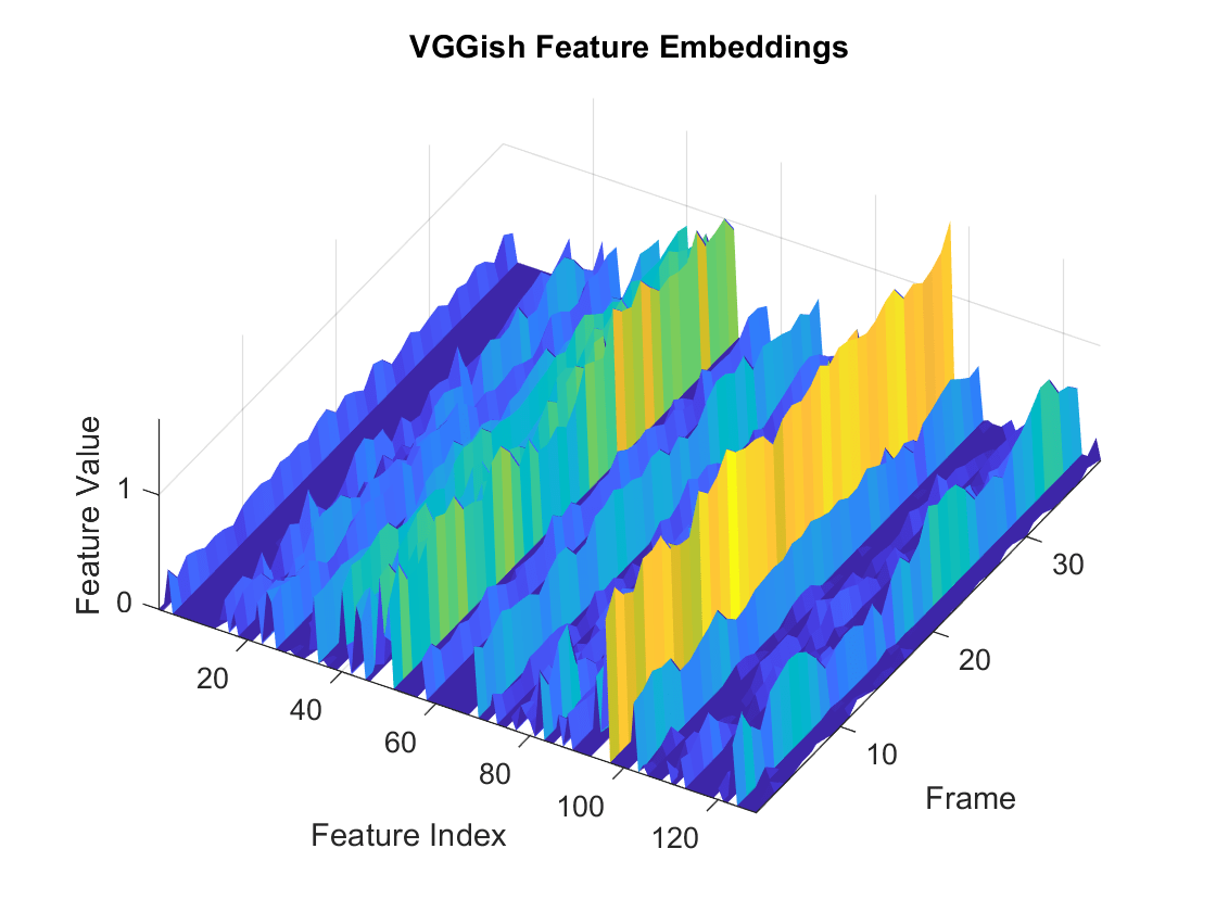
To increase the resolution of VGGish feature embeddings over time, specify the percent overlap between mel spectrograms. Plot the results.
overlapPercentage =75; embeddings = vggishEmbeddings(audioIn,fs,OverlapPercentage=overlapPercentage); surf(embeddings,EdgeColor="none") view([30 65]) axis tight xlabel("Feature Index") ylabel("Frame") zlabel("Feature Value") title("VGGish Feature Embeddings")
Read in an audio file, listen to it, and then extract VGGish feature embeddings from the audio. Using the vggishEmbeddings function requires installing the pretrained VGGish network. If the network is not installed, the function provides a link to download the pretrained model.
[audioIn,fs] = audioread("Counting-16-44p1-mono-15secs.wav");
sound(audioIn,fs)
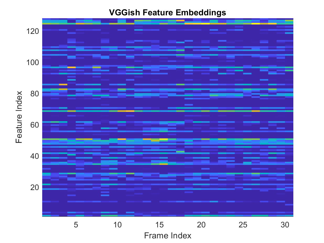
embeddings = vggishEmbeddings(audioIn,fs);Visualize the VGGish feature embeddings over time. Many of the individual features are zero-valued and contain no useful information.
surf(embeddings,EdgeColor="none") view([90,-90]) axis tight xlabel("Feature Index") ylabel("Frame Index") title("VGGish Feature Embeddings")
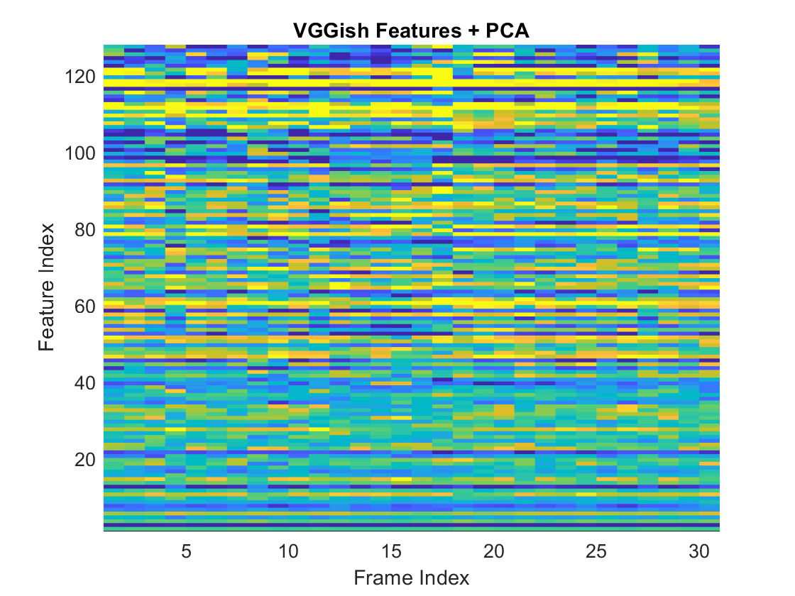
You can apply principal component analysis (PCA) to map the feature vectors into a space that emphasizes variation between the embeddings. Call the vggishEmbeddings function again and specify ApplyPCA as true. Visualize the VGGish feature embeddings after PCA.
embeddings = vggishEmbeddings(audioIn,fs,ApplyPCA=true); surf(embeddings,EdgeColor="none") view([90,-90]) axis tight xlabel("Feature Index") ylabel("Frame Index") title("VGGish Features + PCA")
Download and unzip the air compressor data set. This data set consists of recordings from air compressors in a healthy state or in one of seven faulty states.
zipFile = matlab.internal.examples.downloadSupportFile("audio", ...
    "AirCompressorDataset/AirCompressorDataset.zip");
unzip(zipFile,tempdir)
dataLocation = fullfile(tempdir,"AirCompressorDataset");
Create an audioDatastore object to manage the data and split it into training and validation sets.
ads = audioDatastore(dataLocation,IncludeSubfolders=true, ...
    LabelSource="foldernames");

[adsTrain,adsValidation] = splitEachLabel(ads,0.8);
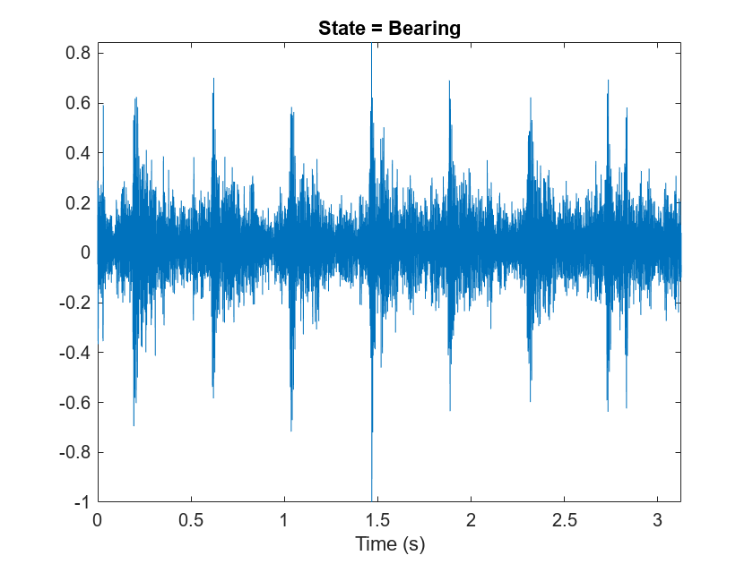
Read an audio file from the datastore. Reset the datastore to return the read pointer to the beginning of the data set. Listen to the audio signal and plot the signal in the time domain.
[x,fileInfo] = read(adsTrain);
fs = fileInfo.SampleRate;

reset(adsTrain)

sound(x,fs)

figure
t = (0:size(x,1)-1)/fs;
plot(t,x)
xlabel("Time (s)")
title("State = " + string(fileInfo.Label))
axis tight
Extract VGGish feature embeddings from the training and validation sets. Using the vggishEmbeddings function requires installing the pretrained VGGish network. If the network is not installed, the function provides a link to download the pretrained model. There are multiple embeddings vectors for each audio file. Replicate the labels so that they are in one-to-one correspondence with the embeddings vectors.
trainFeatures = [];
trainLabels = [];
while hasdata(adsTrain)
    [audioIn,fileInfo] = read(adsTrain);
    features = vggishEmbeddings(audioIn,fileInfo.SampleRate, ...
        OverlapPercentage=75);
    numFeatureVecs = size(features,1);
    trainFeatures = cat(1,trainFeatures,features);
    trainLabels = cat(1,trainLabels,repelem(fileInfo.Label,numFeatureVecs)');
end

classNames = unique(trainLabels);

validationFeatures = [];
validationLabels = [];
segmentsPerFile = zeros(numel(adsValidation.Files), 1);
idx = 1;
while hasdata(adsValidation)
    [audioIn,fileInfo] = read(adsValidation);
    features = vggishEmbeddings(audioIn,fileInfo.SampleRate, ...
        OverlapPercentage=75);
    numFeatureVecs = size(features,1);
    validationFeatures = cat(1,validationFeatures,features);
    validationLabels = cat(1,validationLabels, ...
        repelem(fileInfo.Label,numFeatureVecs)');

    segmentsPerFile(idx) = numFeatureVecs;
    idx = idx + 1;
end
Define a simple network with two fully connected layers.
layers = [
    featureInputLayer(128)
    fullyConnectedLayer(32)
    reluLayer
    fullyConnectedLayer(8)
    softmaxLayer];
To define training options, use trainingOptions (Deep Learning Toolbox).
miniBatchSize = 128;
options = trainingOptions("adam", ...
    MaxEpochs=20, ...
    MiniBatchSize=miniBatchSize, ...
    Shuffle="every-epoch", ...
    ValidationData={validationFeatures,validationLabels}, ...
    ValidationFrequency=50, ...
    Plots="training-progress", ...
    Metrics="accuracy", ...
    Verbose=false);
To train the network, use trainnet.
net = trainnet(trainFeatures,trainLabels,layers,"crossentropy",options)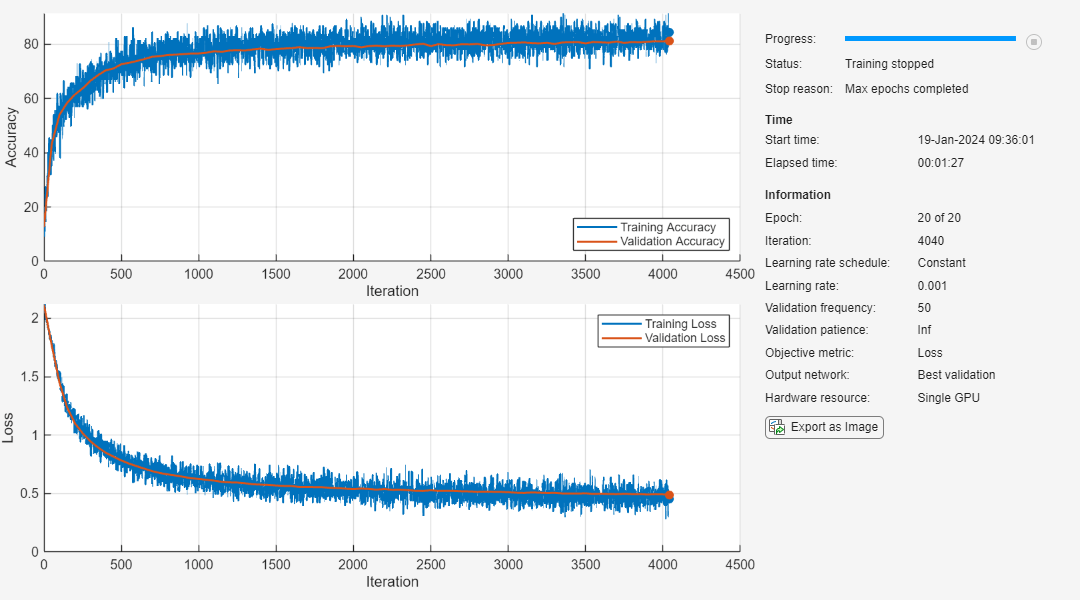
net =
  dlnetwork with properties:

         Layers: [5×1 nnet.cnn.layer.Layer]
    Connections: [4×2 table]
     Learnables: [4×3 table]
          State: [0×3 table]
     InputNames: {'input'}
    OutputNames: {'softmax'}
    Initialized: 1

  View summary with summary.
Each audio file was split into several segments to feed into the network. Combine the predictions for each file in the validation set using a majority-rule decision.
scores = predict(net,validationFeatures);
validationPredictions = scores2label(scores,classNames);

idx = 1;
validationPredictionsPerFile = categorical;
for ii = 1:numel(adsValidation.Files)
    validationPredictionsPerFile(ii,1) = ...
        mode(validationPredictions(idx:idx+segmentsPerFile(ii)-1));
    idx = idx + segmentsPerFile(ii);
end
Visualize the confusion matrix for the validation set.
figure
confusionchart(adsValidation.Labels,validationPredictionsPerFile, ...
    Title=sprintf("Confusion Matrix for Validation Data \nAccuracy = %0.2f %%", ...
    mean(validationPredictionsPerFile==adsValidation.Labels)*100))

Download and unzip the air compressor data set [1]. This data set consists of recordings from air compressors in a healthy state or in one of seven faulty states.
datasetZipFile = matlab.internal.examples.downloadSupportFile("audio","AirCompressorDataset/AirCompressorDataset.zip");
datasetFolder = fullfile(fileparts(datasetZipFile),"AirCompressorDataset");
if ~exist(datasetFolder,"dir")
     unzip(datasetZipFile,fileparts(datasetZipFile));
end
Create an audioDatastore object to manage the data and split it into training and validation sets.
ads = audioDatastore(datasetFolder,IncludeSubfolders=true,LabelSource="foldernames");In this example, you classify signals as either healthy or faulty. Combine all of the faulty labels into a single label. Split the datastore into training and validation sets.
labels = ads.Labels;
labels(labels~=categorical("Healthy")) = categorical("Faulty");
ads.Labels = removecats(labels);

[adsTrain,adsValidation] = splitEachLabel(ads,0.8,0.2);
Extract VGGish feature embeddings from the training set. Each audio file corresponds to multiple VGGish features. Replicate the labels so that they are in one-to-one correspondence with the features. Using the vggishEmbeddings function requires installing the pretrained VGGish network. If the network is not installed, the function provides a link to download the pretrained model.
trainFeatures = [];
trainLabels = [];
for idx = 1:numel(adsTrain.Files)
    [audioIn,fileInfo] = read(adsTrain);
    embeddings = vggishEmbeddings(audioIn,fileInfo.SampleRate);
    trainFeatures = [trainFeatures;embeddings];
    trainLabels = [trainLabels;repelem(fileInfo.Label,size(embeddings,1))'];
end
Train a cubic support vector machine (SVM) using fitcsvm (Statistics and Machine Learning Toolbox). To explore other classifiers and their performances, use Classification Learner (Statistics and Machine Learning Toolbox).
faultDetector = fitcsvm( ...
    trainFeatures, ...
    trainLabels, ...
    KernelFunction="polynomial", ...
    PolynomialOrder=3, ...
    KernelScale="auto", ...
    BoxConstraint=1, ...
    Standardize=true, ...
    ClassNames=categories(trainLabels));
For each file in the validation set:
Extract VGGish feature embeddings.
For each VGGish feature vector in a file, use the trained classifier to predict whether the machine is healthy or faulty.
Take the mode of the predictions for each file.
predictions = [];
for idx = 1:numel(adsValidation.Files)
    [audioIn,fileInfo] = read(adsValidation);

    embeddings = vggishEmbeddings(audioIn,fileInfo.SampleRate);

    predictionsPerFile = categorical(predict(faultDetector,embeddings));

    predictions = [predictions;mode(predictionsPerFile)];
end
Use confusionchart (Statistics and Machine Learning Toolbox) to display the performance of the classifier.
accuracy = sum(predictions==adsValidation.Labels)/numel(adsValidation.Labels);
cc = confusionchart(predictions,adsValidation.Labels);
cc.Title = sprintf("Accuracy = %0.2f %",accuracy*100);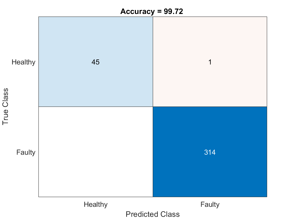
References
[1] Verma, Nishchal K., Rahul Kumar Sevakula, Sonal Dixit, and Al Salour. 2016. “Intelligent Condition Based Monitoring Using Acoustic Signals for Air Compressors.” IEEE Transactions on Reliability 65 (1): 291–309. https://doi.org/10.1109/TR.2015.2459684.
Input Arguments
Name-Value Arguments
Output Arguments
Algorithms
References
[1] Gemmeke, Jort F., Daniel P. W. Ellis, Dylan Freedman, Aren Jansen, Wade Lawrence, R. Channing Moore, Manoj Plakal, and Marvin Ritter. 2017. “Audio Set: An Ontology and Human-Labeled Dataset for Audio Events.” In 2017 IEEE International Conference on Acoustics, Speech and Signal Processing (ICASSP), 776–80. New Orleans, LA: IEEE. https://doi.org/10.1109/ICASSP.2017.7952261.
[2] Hershey, Shawn, Sourish Chaudhuri, Daniel P. W. Ellis, Jort F. Gemmeke, Aren Jansen, R. Channing Moore, Manoj Plakal, et al. 2017. “CNN Architectures for Large-Scale Audio Classification.” In 2017 IEEE International Conference on Acoustics, Speech and Signal Processing (ICASSP), 131–35. New Orleans, LA: IEEE. https://doi.org/10.1109/ICASSP.2017.7952132.
Extended Capabilities
Version History
Introduced in R2022a