Modulation Classification with Deep Learning

This example uses:

This example shows how to use a convolutional neural network (CNN) for modulation classification. You generate synthetic, channel-impaired waveforms. Using the generated waveforms as training data, you train a CNN for modulation classification. You then test the CNN with software-defined radio (SDR) hardware and over-the-air signals.

Predict Modulation Type Using CNN

The trained CNN in this example recognizes these eight digital and three analog modulation types:

Binary phase shift keying (BPSK)
Quadrature phase shift keying (QPSK)
8-ary phase shift keying (8-PSK)
16-ary quadrature amplitude modulation (16-QAM)
64-ary quadrature amplitude modulation (64-QAM)
4-ary pulse amplitude modulation (PAM4)
Gaussian frequency shift keying (GFSK)
Continuous phase frequency shift keying (CPFSK)
Broadcast FM (B-FM)
Double sideband amplitude modulation (DSB-AM)
Single sideband amplitude modulation (SSB-AM)

modulationTypes = categorical(sort(["BPSK", "QPSK", "8PSK", ...
  "16QAM", "64QAM", "PAM4", "GFSK", "CPFSK", ...
  "B-FM", "DSB-AM", "SSB-AM"]));

First, load the trained network. For details on network training, see the Training a CNN section.

load trainedModulationClassificationNetwork
trainedNet

trainedNet = 
  dlnetwork with properties:

         Layers: [19×1 nnet.cnn.layer.Layer]
    Connections: [18×2 table]
     Learnables: [22×3 table]
          State: [10×3 table]
     InputNames: {'Input Layer'}
    OutputNames: {'SoftMax'}
    Initialized: 1

  View summary with summary.

The trained CNN takes 1024 channel-impaired samples and predicts the modulation type of each frame. Generate several PAM4 frames that are impaired with Rician multipath fading, center frequency and sampling time drift, and AWGN. Use following function to generate synthetic signals to test the CNN. Then use the CNN to predict the modulation type of the frames.

randi: Generate random bits
pammod (Communications Toolbox) PAM4-modulate the bits
rcosdesign (Signal Processing Toolbox): Design a square-root raised cosine pulse shaping filter
filter: Pulse shape the symbols
comm.RicianChannel (Communications Toolbox): Apply Rician multipath channel
comm.PhaseFrequencyOffset (Communications Toolbox): Apply phase and/or frequency shift due to clock offset
interp1: Apply timing drift due to clock offset
awgn (Communications Toolbox): Add AWGN

% Set the random number generator to a known state to be able to regenerate
% the same frames every time the simulation is run
rng(123456)
% Random bits
d = randi([0 3], 1024, 1);
% PAM4 modulation
syms = pammod(d,4);
% Square-root raised cosine filter
filterCoeffs = rcosdesign(0.35,4,8);
tx = filter(filterCoeffs,1,upsample(syms,8));

% Channel
SNR = 30;
maxOffset = 5;
fc = 902e6;
fs = 200e3;
multipathChannel = comm.RicianChannel(...
  'SampleRate', fs, ...
  'PathDelays', [0 1.8 3.4] / 200e3, ...
  'AveragePathGains', [0 -2 -10], ...
  'KFactor', 4, ...
  'MaximumDopplerShift', 4);

frequencyShifter = comm.PhaseFrequencyOffset(...
  'SampleRate', fs);

% Apply an independent multipath channel
reset(multipathChannel)
outMultipathChan = multipathChannel(tx);

% Determine clock offset factor
clockOffset = (rand() * 2*maxOffset) - maxOffset;
C = 1 + clockOffset / 1e6;

% Add frequency offset
frequencyShifter.FrequencyOffset = -(C-1)*fc;
outFreqShifter = frequencyShifter(outMultipathChan);

% Add sampling time drift
t = (0:length(tx)-1)' / fs;
newFs = fs * C;
tp = (0:length(tx)-1)' / newFs;
outTimeDrift = interp1(t, outFreqShifter, tp);

% Add noise
rx = awgn(outTimeDrift,SNR,0);

% Frame generation for classification
unknownFrames = helperModClassGetNNFrames(rx);

% Classification
scores1 = predict(trainedNet,unknownFrames);
prediction1 = scores2label(scores1,modulationTypes);

Return the classifier predictions, which are analogous to hard decisions. The network correctly identifies the frames as PAM4 frames. For details on the generation of the modulated signals, see helperModClassGetModulator function.

prediction1

prediction1 = 7×1 categorical
     PAM4 
     PAM4 
     PAM4 
     PAM4 
     PAM4 
     PAM4 
     PAM4

The classifier also returns a vector of scores for each frame. The score corresponds to the probability that each frame has the predicted modulation type. Plot the scores.

helperModClassPlotScores(scores1,modulationTypes)

Before we can use a CNN for modulation classification, or any other task, we first need to train the network with known (or labeled) data. The first part of this example shows how to use Communications Toolbox™ features, such as modulators, filters, and channel impairments, to generate synthetic training data. The second part focuses on defining, training, and testing the CNN for the task of modulation classification. The third part tests the network performance with over-the-air signals using software defined radio (SDR) platforms.

Waveform Generation for Training

Generate 10,000 frames for each modulation type, where 80% is used for training, 10% is used for validation and 10% is used for testing. We use training and validation frames during the network training phase. Final classification accuracy is obtained using test frames. Each frame is 1024 samples long and has a sample rate of 200 kHz. For digital modulation types, eight samples represent a symbol. The network makes each decision based on single frames rather than on multiple consecutive frames (as in video). Assume a center frequency of 902 MHz and 100 MHz for the digital and analog modulation types, respectively.

To run this example quickly, use the trained network and generate a small number of training frames. To train the network on your computer, choose the "Train network now" option (i.e. set trainNow to true).

trainNow = false;
if trainNow == true
  numFramesPerModType = 10000;
else
  numFramesPerModType = 200;
end
percentTrainingSamples = 80;
percentValidationSamples = 10;
percentTestSamples = 10;

sps = 8;                % Samples per symbol
spf = 1024;             % Samples per frame
fs = 200e3;             % Sample rate
fc = [902e6 100e6];     % Center frequencies

Create Channel Impairments

Pass each frame through a channel with

AWGN
Rician multipath fading
Clock offset, resulting in center frequency offset and sampling time drift

Because the network in this example makes decisions based on single frames, each frame must pass through an independent channel.

AWGN

The channel adds AWGN with an SNR of 30 dB. Implement the channel using awgn (Communications Toolbox) function.

Rician Multipath

The channel passes the signals through a Rician multipath fading channel using the comm.RicianChannel (Communications Toolbox) System object™. Assume a delay profile of [0 1.8 3.4] samples with corresponding average path gains of [0 -2 -10] dB. The K-factor is 4 and the maximum Doppler shift is 4 Hz, which is equivalent to a walking speed at 902 MHz. Implement the channel with the following settings.

Clock Offset

Clock offset occurs because of the inaccuracies of internal clock sources of transmitters and receivers. Clock offset causes the center frequency, which is used to downconvert the signal to baseband, and the digital-to-analog converter sampling rate to differ from the ideal values. The channel simulator uses the clock offset factor $C$ , expressed as $C = 1 + \frac{Δ_{clock}}{10^{6}}$ , where $Δ_{clock}$ is the clock offset. For each frame, the channel generates a random $Δ_{clock}$ value from a uniformly distributed set of values in the range [ ${- \max Δ}_{clock}$ ${\max Δ}_{clock}$ ], where ${\max Δ}_{clock}$ is the maximum clock offset. Clock offset is measured in parts per million (ppm). For this example, assume a maximum clock offset of 5 ppm.

maxDeltaOff = 5;
deltaOff = (rand()*2*maxDeltaOff) - maxDeltaOff;
C = 1 + (deltaOff/1e6);

Frequency Offset

Subject each frame to a frequency offset based on clock offset factor $C$ and the center frequency. Implement the channel using comm.PhaseFrequencyOffset (Communications Toolbox).

Sampling Rate Offset

Subject each frame to a sampling rate offset based on clock offset factor $C$ . Implement the channel using the interp1 function to resample the frame at the new rate of $C \times f_{s}$ .

Combined Channel

Use the helperModClassTestChannel object to apply all three channel impairments to the frames.

channel = helperModClassTestChannel(...
  'SampleRate', fs, ...
  'SNR', SNR, ...
  'PathDelays', [0 1.8 3.4] / fs, ...
  'AveragePathGains', [0 -2 -10], ...
  'KFactor', 4, ...
  'MaximumDopplerShift', 4, ...
  'MaximumClockOffset', 5, ...
  'CenterFrequency', 902e6)

channel = 
  helperModClassTestChannel with properties:

                    SNR: 30
        CenterFrequency: 902000000
             SampleRate: 200000
             PathDelays: [0 9.0000e-06 1.7000e-05]
       AveragePathGains: [0 -2 -10]
                KFactor: 4
    MaximumDopplerShift: 4
     MaximumClockOffset: 5

You can view basic information about the channel using the info object function.

chInfo = info(channel)

chInfo = struct with fields:
               ChannelDelay: 6
     MaximumFrequencyOffset: 4510
    MaximumSampleRateOffset: 1

Waveform Generation

Create a loop that generates channel-impaired frames for each modulation type and stores the frames with their corresponding labels in MAT files. By saving the data into files, you eliminate the need to generate the data every time you run this example. You can also share the data more effectively.

Remove a random number of samples from the beginning of each frame to remove transients and to make sure that the frames have a random starting point with respect to the symbol boundaries.

% Set the random number generator to a known state to be able to regenerate
% the same frames every time the simulation is run
rng(12)
tic
numModulationTypes = length(modulationTypes);
channelInfo = info(channel);
transDelay = 50;
pool = getPoolSafe();
if ~isa(pool,"parallel.ClusterPool")
  dataDirectory = fullfile(tempdir,"ModClassDataFiles");
else
  dataDirectory = uigetdir("","Select network location to save data files");
end
disp("Data file directory is " + dataDirectory)

Data file directory is C:\TEMP\ModClassDataFiles

fileNameRoot = "frame";

% Check if data files exist
dataFilesExist = false;
if exist(dataDirectory,'dir')
  files = dir(fullfile(dataDirectory,sprintf("%s*",fileNameRoot)));
  if length(files) == numModulationTypes*numFramesPerModType
    dataFilesExist = true;
  end
end

if ~dataFilesExist
  disp("Generating data and saving in data files...")
  [success,msg,msgID] = mkdir(dataDirectory);
  if ~success
    error(msgID,msg)
  end
  for modType = 1:numModulationTypes
    elapsedTime = seconds(toc);
    elapsedTime.Format = 'hh:mm:ss';
    fprintf('%s - Generating %s frames\n', ...
      elapsedTime, modulationTypes(modType))
    
    label = modulationTypes(modType);
    numSymbols = (numFramesPerModType / sps);
    dataSrc = helperModClassGetSource(modulationTypes(modType), sps, 2*spf, fs);
    modulator = helperModClassGetModulator(modulationTypes(modType), sps, fs);
    if contains(char(modulationTypes(modType)), {'B-FM','DSB-AM','SSB-AM'})
      % Analog modulation types use a center frequency of 100 MHz
      channel.CenterFrequency = 100e6;
    else
      % Digital modulation types use a center frequency of 902 MHz
      channel.CenterFrequency = 902e6;
    end
    
    for p=1:numFramesPerModType
      % Generate random data
      x = dataSrc();
      
      % Modulate
      y = modulator(x);
      
      % Pass through independent channels
      rxSamples = channel(y);
      
      % Remove transients from the beginning, trim to size, and normalize
      frame = helperModClassFrameGenerator(rxSamples, spf, spf, transDelay, sps);
      
      % Save data file
      fileName = fullfile(dataDirectory,...
        sprintf("%s%s%03d",fileNameRoot,modulationTypes(modType),p));
      save(fileName,"frame","label")
    end
  end
else
  disp("Data files exist. Skip data generation.")
end

Generating data and saving in data files...

00:00:00 - Generating 16QAM frames
00:00:01 - Generating 64QAM frames
00:00:02 - Generating 8PSK frames
00:00:04 - Generating B-FM frames
00:00:05 - Generating BPSK frames
00:00:07 - Generating CPFSK frames
00:00:08 - Generating DSB-AM frames
00:00:10 - Generating GFSK frames
00:00:11 - Generating PAM4 frames
00:00:12 - Generating QPSK frames
00:00:14 - Generating SSB-AM frames

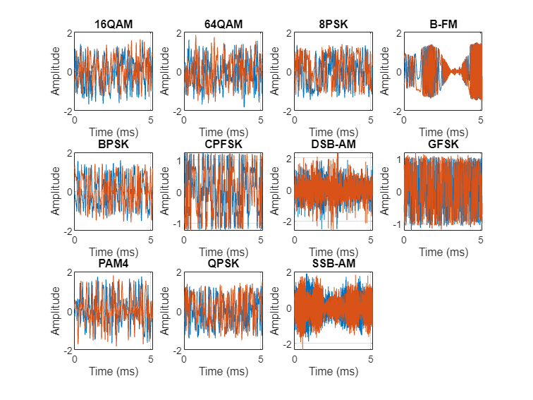
% Plot the amplitude of the real and imaginary parts of the example frames
% against the sample number
helperModClassPlotTimeDomain(dataDirectory,modulationTypes,fs)

% Plot the spectrogram of the example frames
helperModClassPlotSpectrogram(dataDirectory,modulationTypes,fs,sps)

Create a Datastore

Use a signalDatastore object to manage the files that contain the generated complex waveforms. Datastores are especially useful when each individual file fits in memory, but the entire collection does not necessarily fit.

frameDS = signalDatastore(dataDirectory,'SignalVariableNames',["frame","label"]);

Split into Training, Validation, and Test

Next divide the frames into training, validation, and test data. See helperModClassSplitData for details.

splitPercentages = [percentTrainingSamples,percentValidationSamples,percentTestSamples];
[trainDS,validDS,testDS] = helperModClassSplitData(frameDS,splitPercentages);

Import Data into Memory

Neural network training is iterative. At every iteration, the datastore reads data from files and transforms the data before updating the network coefficients. If the data fits into the memory of your computer, importing the data from the files into the memory enables faster training by eliminating this repeated read from file and transform process. Instead, the data is read from the files and transformed once.

Import all the data in the files into memory. The files have two variables: frame and label and each read call to the datastore returns a cell array, where the first element is the frame and the second element is the label. Use the transform functions helperModClassReadFrame and helperModClassReadLabel to read frames and labels. Use readall with "UseParallel" option set to true to enable parallel processing of the transform functions, in case you have Parallel Computing Toolbox™ license. Since readall function, by default, concatenates the output of the read function over the first dimension, return the frames in a cell array and manually concatenate over the 4th dimension.

% Read the training and validation frames into the memory
pctExists = parallelComputingLicenseExists();
trainFrames = transform(trainDS, @helperModClassReadFrame);
rxTrainFrames = readall(trainFrames,"UseParallel",pctExists);
validFrames = transform(validDS, @helperModClassReadFrame);
rxValidFrames = readall(validFrames,"UseParallel",pctExists);

% Read the training and validation labels into the memory
trainLabels = transform(trainDS, @helperModClassReadLabel);
rxTrainLabels = readall(trainLabels,"UseParallel",pctExists);
validLabels = transform(validDS, @helperModClassReadLabel);
rxValidLabels = readall(validLabels,"UseParallel",pctExists);

Train the CNN

This example uses a CNN that consists of five convolution layers and one fully connected layer. Each convolution layer except the last is followed by a batch normalization layer, rectified linear unit (ReLU) activation layer, and max pooling layer. In the last convolution layer, the max pooling layer is replaced with an global average pooling layer. The output layer has softmax activation. For network design guidance, see Deep Learning Tips and Tricks.

modClassNet = helperModClassCNN(modulationTypes,sps,spf);

Next configure TrainingOptionsSGDM to use an SGDM solver with a mini-batch size of 1024. Set the maximum number of epochs to 20, since a larger number of epochs provides no further training advantage. By default, the 'ExecutionEnvironment' property is set to 'auto', where the trainNetwork function uses a GPU if one is available or uses the CPU, if not. To use the GPU, you must have a Parallel Computing Toolbox license. Set the initial learning rate to $3 x 10^{- 1}$ . Reduce the learning rate by a factor of 0.75 every 6 epochs. Set 'Plots' to 'training-progress' to plot the training progress. On an NVIDIA® GeForce RTX 3080 GPU, the network takes approximately 3 minutes to train.

maxEpochs = 20;
miniBatchSize = 1024;
trainingPlots = "none";
metrics = [];
verbose = true;
validationFrequency = floor(numel(rxTrainLabels)/miniBatchSize);
options = trainingOptions('sgdm', ...
  InitialLearnRate = 3e-1, ...
  MaxEpochs = maxEpochs, ...
  MiniBatchSize = miniBatchSize, ...
  Shuffle = 'every-epoch', ...
  Plots = trainingPlots, ...
  Verbose = verbose, ...
  ValidationData = {rxValidFrames,rxValidLabels}, ...
  ValidationFrequency = validationFrequency, ...
  ValidationPatience = 5, ...
  Metrics = metrics, ...
  LearnRateSchedule = 'piecewise', ...
  LearnRateDropPeriod = 6, ...
  LearnRateDropFactor = 0.75, ...
  OutputNetwork='best-validation-loss');

Either train the network or use the already trained network. By default, this example uses the trained network.

if trainNow == true
  elapsedTime = seconds(toc);
  elapsedTime.Format = 'hh:mm:ss';
  fprintf('%s - Training the network\n', elapsedTime)
  trainedNet = trainnet(rxTrainFrames,rxTrainLabels,modClassNet,"crossentropy",options);
else
  load trainedModulationClassificationNetwork
end

The following plot shows an example run with trainingPlots set to "Training progress", metric set to "Accuracy", and verbose set to false. The network converges in about 20 epochs to about 97% accuracy.

Evaluate the trained network by obtaining the classification accuracy for the test frames. The results show that the network achieves about 96% accuracy for this group of waveforms.

elapsedTime = seconds(toc);
elapsedTime.Format = 'hh:mm:ss';
fprintf('%s - Classifying test frames\n', elapsedTime)

00:00:32 - Classifying test frames

% Read the test frames into the memory
testFrames = transform(testDS, @helperModClassReadFrame);
rxTestFrames = readall(testFrames,"UseParallel",pctExists);

% Read the test labels into the memory
testLabels = transform(testDS, @helperModClassReadLabel);
rxTestLabels = readall(testLabels,"UseParallel",pctExists);

scores = predict(trainedNet,cat(3,rxTestFrames{:}));
rxTestPred = scores2label(scores,modulationTypes);
testAccuracy = mean(rxTestPred == rxTestLabels);
disp("Test accuracy: " + testAccuracy*100 + "%")

Test accuracy: 97.7273%

Plot the confusion matrix for the test frames. As the matrix shows, the network confuses 16-QAM and 64-QAM frames. This problem is expected since each frame carries only 128 symbols and 16-QAM is a subset of 64-QAM. The network also confuses DSB-AM and SSB-AM frames, since the SSB-AM signals contains exactly half the spectrum of the DSB-AM signals.

figure
cm = confusionchart(rxTestLabels, rxTestPred);
cm.Title = 'Confusion Matrix for Test Data';
cm.RowSummary = 'row-normalized';
cm.Parent.Position = [cm.Parent.Position(1:2) 950 550];

Test with SDR

Test the performance of the trained network with over-the-air signals using the helperModClassSDRTest function. To perform this test, you must have dedicated SDRs for transmission and reception. You can use two ADALM-PLUTO radios, or one ADALM-PLUTO radio for transmission and one USRP® radio for reception. You must Install Support Package for Analog Devices ADALM-PLUTO Radio (Communications Toolbox). If you are using a USRP® radio, you must also Install Communications Toolbox Support Package for USRP Radio (Communications Toolbox). The helperModClassSDRTest function uses the same modulation functions as used for generating the training signals, and then transmits them using an ADALM-PLUTO radio. Instead of simulating the channel, capture the channel-impaired signals using the SDR that is configured for signal reception (ADALM-PLUTO or USRP® radio). Use the trained network with the same perdict function used previously to predict the modulation type. Running the next code segment produces a confusion matrix and prints out the test accuracy.

radioPlatform = "ADALM-PLUTO";

switch radioPlatform
  case "ADALM-PLUTO"
    if helperIsPlutoSDRInstalled() == true
      radios = findPlutoRadio();
      if length(radios) >= 2
        helperModClassSDRTest(radios);
      else
        disp('Selected radios not found. Skipping over-the-air test.')
      end
    end
  case {"USRP B2xx","USRP X3xx","USRP N2xx"}
    if (helperIsUSRPInstalled() == true) && (helperIsPlutoSDRInstalled() == true)
      txRadio = findPlutoRadio();
      rxRadio = findsdru();
      switch radioPlatform
        case "USRP B2xx"
          idx = contains({rxRadio.Platform}, {'B200','B210'});
        case "USRP X3xx"
          idx = contains({rxRadio.Platform}, {'X300','X310'});
        case "USRP N2xx"
          idx = contains({rxRadio.Platform}, 'N200/N210/USRP2');
      end
      rxRadio = rxRadio(idx);
      if (length(txRadio) >= 1) && (length(rxRadio) >= 1)
        helperModClassSDRTest(rxRadio);
      else
        disp('Selected radios not found. Skipping over-the-air test.')
      end
    end
end

Selected radios not found. Skipping over-the-air test.

When using two stationary ADALM-PLUTO radios separated by about 2 feet, the network achieves 99% overall accuracy with the following confusion matrix. Results will vary based on experimental setup.

Further Exploration

It is possible to optimize the hyperparameters parameters, such as number of filters, filter size, or optimize the network structure, such as adding more layers, using different activation layers, etc. to improve the accuracy.

Communication Toolbox provides many more modulation types and channel impairments. For more information see Modulation (Communications Toolbox) and Propagation and Channel Models (Communications Toolbox) sections. You can also add standard specific signals with LTE Toolbox, WLAN Toolbox, and 5G Toolbox. You can also add radar signals with Phased Array System Toolbox.

Helper Files

helperModClassGetModulator function provides the MATLAB® functions used to generate modulated signals. You can also explore the following functions and System objects for more details:

Local Functions

function pool = getPoolSafe()
if exist("gcp","file") && license('test','distrib_computing_toolbox')
  pool = gcp;
  if isempty(pool)
    pool = parpool;
  end
else
  pool = [];
end
end

References

O'Shea, T. J., J. Corgan, and T. C. Clancy. "Convolutional Radio Modulation Recognition Networks." Preprint, submitted June 10, 2016. https://arxiv.org/abs/1602.04105
O'Shea, T. J., T. Roy, and T. C. Clancy. "Over-the-Air Deep Learning Based Radio Signal Classification." IEEE Journal of Selected Topics in Signal Processing. Vol. 12, Number 1, 2018, pp. 168–179.
Liu, X., D. Yang, and A. E. Gamal. "Deep Neural Network Architectures for Modulation Classification." Preprint, submitted January 5, 2018. https://arxiv.org/abs/1712.00443v3