Lane Detection in Lidar Data Using Deep Learning

This example shows how to detect lanes in point clouds using a lidar lane detection network utilizing global feature correlator (LLDN-GFC) [1], which detects lanes in point clouds using intensity values. In this example, you:

• Configure a data set for training, validation, and testing of the lane detection network.

• Create an LLDN-GFC lidar lane detector and train the lane detection network.

• Evaluate the trained detector.

This example also provides a pretrained lane detector to detect lanes in point clouds. The pretrained network has been trained on the KAIST-Lane (K-Lane) data set [1], captured using a 64-channel Ouster® lidar sensor.

Download Data Set

This example uses a subset of the K-Lane data set that contains 900 unorganized point clouds. This data set has been collected using a lidar mounted on the ego vehicle. The point clouds are stored in PCD format, and their corresponding ground truth data is stored in the GroundTruthLaneData.mat file. The file contains lane boundary point information for six classes. The size of the dataset is 1.2 GB.

Download and unzip a ZIP file containing the subset of the K-Lane dataset.

outputFolder = fullfile(tempdir,"KLane");
if ~exist(outputFolder,'file')
    mkdir(outputFolder);
end

dataFilename = "KLaneData.zip";
url = "https://ssd.mathworks.com/supportfiles/driving/data/" + dataFilename;
filePath = fullfile(outputFolder,dataFilename);
if ~isfile(filePath)
    websave(filePath,url)
end
unzip(filePath,outputFolder)
dataset = fullfile(outputFolder,"KLaneData");

Depending on your internet connection, the download process can take some time. The code suspends MATLAB® execution until the download process is complete. Alternatively, you can download the data set to your local disk using your web browser and extract the file. If you do so, change the outputFolder variable in the code to the location of the downloaded file.

Load Data

Create file datastores for training and test sets as fileDatastore objects. Each datastore loads the PCD files from the specified path using the pcread function.

% File path to training data.
trainDataPath = fullfile(dataset,"Train","lidarPointCloudData");
ldsTrain = fileDatastore(trainDataPath,"ReadFcn",@(x) pcread(x));

% File path to test data.
testDataPath = fullfile(dataset,"Test","lidarPointCloudData");
ldsTest = fileDatastore(testDataPath,"ReadFcn",@(x) pcread(x));

Create an array datastore as an arrayDatastore object, and load the ground truth labels into it.

Data = load(fullfile(dataset,"Train","GroundTruthLaneData.mat"));
gTruth = Data.gTruth;

trainLabels = arrayDatastore(gTruth);

Load the ground truth labels for the test data.

testData = load(fullfile(dataset,"Test","GroundTruthLaneData.mat"));
testLabels = testData.gTruth;

Create training and validation data sets.

trainRatio = 0.7;
rng(10)
shuffledIndices = randperm(height(gTruth));
idx = floor(trainRatio*length(shuffledIndices));

trainingIdx = shuffledIndices(1:idx);
validationIdx = shuffledIndices(idx+1:length(shuffledIndices));

trainingData = subset(ldsTrain,trainingIdx);
trainingLabels = subset(trainLabels,trainingIdx); 

validationData = subset(ldsTrain,validationIdx);
validationLabels = subset(trainLabels,validationIdx);

Combine the point cloud training data and its ground truth information into a single datastore by using the combine function. Repeat the process for the validation data.

trainingCDS = combine(trainingData,trainingLabels);
validationCDS = combine(validationData,validationLabels);

Read and display the first point cloud in the data set.

data = read(trainingCDS);
ptCld = data{1};
labels = data{2};
helperDisplayLanes(ptCld,labels)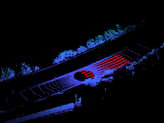

reset(trainingCDS)

Create Lidar Lane Detection Network

In this example, you create an LLDN-GFC network using the lidarLaneDetector function. The function requires you to specify these inputs that parameterize the network:

• Class names

• Detector name

• Point cloud range

Specify the class names of the lanes.

classNames = gTruth.Properties.VariableNames;

Specify the range of the input point cloud.

xMin = 0.02;    % Minimum value along x-axis.
yMin = -11.52;  % Minimum value along y-axis.
zMin = -3.0;    % Minimum value along z-axis.
xMax = 46.08;   % Maximum value along x-axis.
yMax = 11.52;   % Maximum value along y-axis.
zMax = 1.5;     % Maximum value along z-axis.
pointCloudRange = [xMin xMax yMin yMax zMin zMax];

Create a lane detector by using the lidarLaneDetector function and specify the point cloud range.

detector = lidarLaneDetector("lldn-gfc-untrained",classNames,PointCloudRange=pointCloudRange);

Specify Training Options

Specify the network training parameters using the trainingOptions (Deep Learning Toolbox) function. Set CheckpointPath to a temporary location to enable you to save of partially trained detectors during the training process. If training is interrupted, you can resume training from the saved checkpoint.

Train the detector using a CPU or GPU. Using a GPU requires Parallel Computing Toolbox™ and a CUDA® enabled NVIDIA® GPU. For more information, see GPU Computing Requirements (Parallel Computing Toolbox) (Parallel Computing Toolbox). To automatically detect if you have a GPU available, set executionEnvironment to "auto". If you do not have a GPU, or do not want to use one for training, set executionEnvironment to "cpu". To ensure the use of a GPU for training, set executionEnvironment to "gpu".

options = trainingOptions("adam", ...
    InitialLearnRate=0.0001, ...
    MiniBatchSize=4, ...
    MaxEpochs=30, ...
    DispatchInBackground=false, ...
    VerboseFrequency=20, ...
    ValidationFrequency=10, ...
    CheckpointPath=tempdir, ...
    ExecutionEnvironment="auto", ...
    ValidationData=validationCDS);

Train Lidar Lane Detector

Use the trainLidarLaneDetector function to train the LLDN-GFC detector. When running this example on an NVIDIA Titan RTX™ GPU with 24 GB of memory, network training required approximately 6 hours for 30 epochs. The training time can vary depending on the hardware you use. Instead of training the network, you can use a pretrained LLDN-GFC detector.

If you want to use the pretrained network, set the doTraining to false. If you want to train the detector on the training data, set the doTraining to true.

doTraining = false;
if doTraining       
    % Train the lidarLaneDetector.
    [detector,info] = trainLidarLaneDetector(trainingCDS,detector,options);
else
    % Load the pretrained detector for the example.
    detector = lidarLaneDetector("lldn-gfc-klane");
end

Generate Detections

Read the point cloud data from a test sample, and run the trained detector to get detections and labels.

pointCloud = read(ldsTest);
[laneDetections,labels] = detect(detector,pointCloud);
reset(ldsTest)

Display the point cloud with the detected lanes.

figure
helperDisplayLanes(pointCloud,laneDetections,testLabels(1,:))

Evaluate Detector Using Test Set

Evaluate the trained lane detector on a set of point clouds to measure the performance using the evaluate function. For this example, use the F1 score, precision, and recall metrics to evaluate the performance.

Run the detector on the entire set of point clouds.

detectionResults = detect(detector,ldsTest);

Evaluate the object detector using the F1 score, precision, and recall metrics.

metrics = evaluate(detector,detectionResults,testLabels);
disp(metrics)

       Accuracy: 0.9819
     ClsF1Score: 0.8811
    ConfF1Score: 0.9120
      Precision: 0.8736
         Recall: 0.8955

Helper Functions

helperDisplayLanes — Displays the specified point cloud with lanes colored based on the specified lane labels.

function helperDisplayLanes(ptCld,laneLabels,varargin)
% Display the point cloud with colored lanes.
    figure
    ax = pcshow(ptCld);
    set(ax,XLim=[-100 100],YLim=[-40 40])
    zoom(ax,2.5)
    axis off
    if istable(laneLabels)
        laneBoundaryPoints = processLabelsForVisualization(laneLabels);
    else
        laneBoundaryPoints = laneLabels;
    end
    hold on
    plot3(laneBoundaryPoints(:,1),laneBoundaryPoints(:,2),laneBoundaryPoints(:,3) ,"*",MarkerSize=2,Color="r")
    if nargin == 3
        gtruthPoints = varargin{1};
        gtruthPoints = processLabelsForVisualization(gtruthPoints);
    plot3(gtruthPoints(:,1),gtruthPoints(:,2),gtruthPoints(:,3),"*",MarkerSize=3,Color="g")
    end
end

function laneBoundaryPoints = processLabelsForVisualization(laneBoundaryPoints)
    columnNames = laneBoundaryPoints.Properties.VariableNames;
    % Remove the first column if it has the Time information.
    if isequal(columnNames{1},"Time")
        laneBoundaryPoints = laneBoundaryPoints(:,2:end);
    end
    laneBoundaryPoints = cellfun(@(x) vertcat(x{:}),{table2cell(laneBoundaryPoints)},UniformOutput=false);
    laneBoundaryPoints = laneBoundaryPoints{1};
end

References

[1] Paek, Dong-Hee, Seung-Hyun Kong, and Kevin Tirta Wijaya. “K-Lane: Lidar Lane Dataset and Benchmark for Urban Roads and Highways.” In 2022 IEEE/CVF Conference on Computer Vision and Pattern Recognition Workshops (CVPRW), 4449–58. New Orleans, LA, USA: IEEE, 2022. https://doi.org/10.1109/CVPRW56347.2022.00491.