gamultiobj
Encuentre el frente de Pareto de múltiples funciones de aptitud utilizando un algoritmo genético
Sintaxis
Descripción
x = gamultiobj(fun,nvars)x en la Frente de Pareto de las funciones objetivo definidas en fun. nvars es la dimensión del problema de optimización (número de variables de decisión). La solución x es local, lo que significa que podría no estar en el frente global de Pareto.
Nota
En Pasar parámetros adicionales se explica cómo pasar parámetros adicionales a la función objetivo y a las funciones de restricción no lineales, si fuera necesario.
x = gamultiobj(fun,nvars,A,b,Aeq,beq)x sujeto a las igualdades lineales y las desigualdades lineales , ver Restricciones de igualdad lineales. (Establezca A = [] y b = [] si no existen desigualdades). gamultiobj admite restricciones lineales solo para la opción PopulationType predeterminada ('doubleVector').
x = gamultiobj(fun,nvars,A,b,Aeq,beq,lb,ub)x de modo que se encuentre un conjunto de Pareto local en el rango lb ≤ x ≤ ub, consulte Restricciones de límite. Utilice matrices vacías para Aeq y beq si no existen restricciones de igualdad lineales. gamultiobj admite restricciones de límites solo para la opción PopulationType predeterminada ('doubleVector').
x = gamultiobj(fun,nvars,A,b,Aeq,beq,lb,ub,nonlcon)nonlcon . La función nonlcon acepta x y devuelve los vectores c y ceq, que representan las desigualdades e igualdades no lineales respectivamente. gamultiobj minimiza fun de modo que c(x) ≤ 0 y ceq(x) = 0. (Establezca lb = [] y ub = [] si no existen límites). gamultiobj admite restricciones no lineales solo para la opción PopulationType predeterminada ('doubleVector').
x = gamultiobj(fun,nvars,A,b,Aeq,beq,lb,ub,options)x = gamultiobj(fun,nvars,A,b,Aeq,beq,lb,ub,nonlcon,options)x con los parámetros de optimización predeterminados reemplazados por valores en options . Crea options utilizando optimoptions (recomendado) o una estructura.
x = gamultiobj(fun,nvars,A,b,Aeq,beq,lb,ub,nonlcon,intcon)x = gamultiobj(fun,nvars,A,b,Aeq,beq,lb,ub,nonlcon,intcon,options)intcon tomen valores enteros.
Nota
Cuando hay restricciones de números enteros, gamultiobj no acepta restricciones de igualdad no lineal, solo restricciones de desigualdad no lineal.
Ejemplos
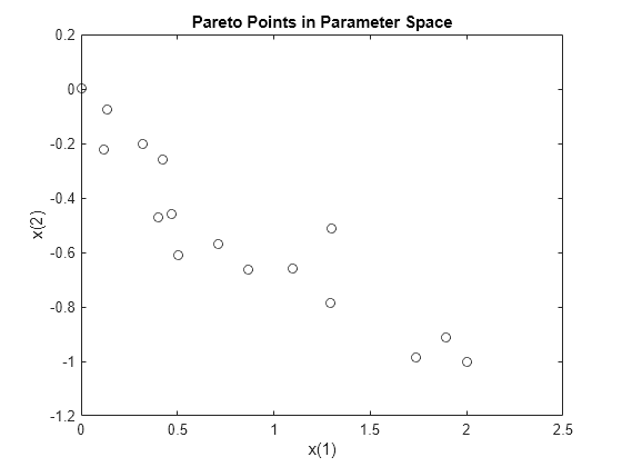
Encuentre el frente de Pareto para un problema multiobjetivo simple. Hay dos objetivos y dos variables de decisión x .
fitnessfcn = @(x)[norm(x)^2,0.5*norm(x(:)-[2;-1])^2+2];
Encuentre el frente de Pareto para esta función objetivo.
rng default % For reproducibility
x = gamultiobj(fitnessfcn,2);
gamultiobj stopped because the average change in the spread of Pareto solutions is less than options.FunctionTolerance.
Representar los puntos solución.
plot(x(:,1),x(:,2),'ko')
xlabel('x(1)')
ylabel('x(2)')
title('Pareto Points in Parameter Space')
\\7\7Para ver el efecto de una restricción lineal en este problema, consulte Problema multiobjetivo con restricción lineal.
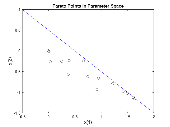
Este ejemplo muestra cómo encontrar el frente de Pareto para un problema multiobjetivo en presencia de una restricción lineal.
Hay dos funciones objetivo y dos variables de decisión x .
fitnessfcn = @(x)[norm(x)^2,0.5*norm(x(:)-[2;-1])^2+2];
La restricción lineal es .
A = [1,1];
b = 1/2;
Encuentra el frente de Pareto.
rng default % For reproducibility
x = gamultiobj(fitnessfcn,2,A,b);
gamultiobj stopped because the average change in the spread of Pareto solutions is less than options.FunctionTolerance.
Grafique la solución restringida y la restricción lineal.
plot(x(:,1),x(:,2),'ko')
t = linspace(-1/2,2);
y = 1/2 - t;
hold on
plot(t,y,'b--')
xlabel('x(1)')
ylabel('x(2)')
title('Pareto Points in Parameter Space')
hold off
Para ver el efecto de eliminar la restricción lineal de este problema, consulte Problema multiobjetivo simple.
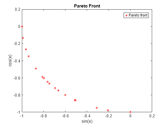
Encuentre el frente de Pareto para las dos funciones de aptitud sin(x) y cos(x) en el intervalo .
fitnessfcn = @(x)[sin(x),cos(x)];
nvars = 1;
lb = 0;
ub = 2*pi;
rng default % for reproducibility
x = gamultiobj(fitnessfcn,nvars,[],[],[],[],lb,ub)
gamultiobj stopped because the average change in the spread of Pareto solutions is less than options.FunctionTolerance.
x = 18×1

    4.7124
    4.7124
    3.1415
    3.6733
    3.9845
    3.4582
    3.9098
    4.4409
    4.0846
    3.8686
      ⋮
Grafica la solución. gamultiobj encuentra puntos a lo largo de todo el frente de Pareto.
plot(sin(x),cos(x),'r*')
xlabel('sin(x)')
ylabel('cos(x)')
title('Pareto Front')
legend('Pareto front')
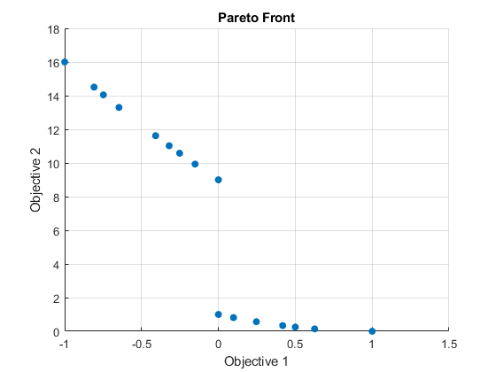
Encuentre y grafique el frente de Pareto para la segunda función de Schaffer de dos objetivos. Esta función tiene un frente de Pareto desconectado.
Copie este código en un archivo de función en su ruta MATLAB®.
function y = schaffer2(x) % y has two columns

% Initialize y for two objectives and for all x
y = zeros(length(x),2);

% Evaluate first objective.
% This objective is piecewise continuous.
for i = 1:length(x)
    if x(i) <= 1
        y(i,1) = -x(i);
    elseif x(i) <=3
        y(i,1) = x(i) -2;
    elseif x(i) <=4
        y(i,1) = 4 - x(i);
    else
        y(i,1) = x(i) - 4;
    end
end

% Evaluate second objective
y(:,2) = (x -5).^2;
Grafica los dos objetivos.
x = -1:0.1:8;
y = schaffer2(x);
plot(x,y(:,1),'r',x,y(:,2),'b');
xlabel x
ylabel 'schaffer2(x)'
legend('Objective 1','Objective 2')
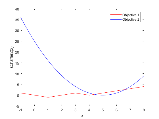
Las dos funciones objetivo compiten por x en los rangos [1,3] y [4,5]. Pero, el frente óptimo de Pareto consta de sólo dos regiones desconectadas, correspondientes a x en los rangos [1,2] y [4,5]. Hay regiones desconectadas porque la región [2,3] es inferior a [4,5]. En ese rango, el objetivo 1 tiene los mismos valores, pero el objetivo 2 es más pequeño.
Establezca límites para mantener a los miembros de la población dentro del rango ![]() .
.
lb = -5;
ub = 10;
Establezca opciones para ver el frente de Pareto mientras se ejecuta gamultiobj.
options = optimoptions('gamultiobj','PlotFcn',@gaplotpareto);
Llame a gamultiobj.
rng default % For reproducibility
[x,fval,exitflag,output] = gamultiobj(@schaffer2,1,[],[],[],[],lb,ub,options);
gamultiobj stopped because it exceeded options.MaxGenerations.
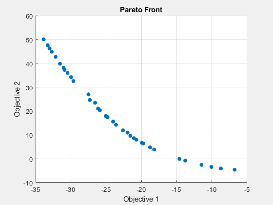
Crear una función de dos objetivos en dos variables del problema.
rng default % For reproducibility
M = diag([-1 -1]) + randn(2)/4; % Two problem variables
fun = @(x)[(x').^2 / 30 + M*x']; % Two objectives
Especifica que la segunda variable debe ser un número entero.
intcon = 2;
Especifique los límites del problema, la función gráfica gaplotpareto y un tamaño de población de 100.
lb = [0 0];
ub = [100 50];
options = optimoptions("gamultiobj","PlotFcn","gaplotpareto",...
    "PopulationSize",100);
Encuentra el conjunto de Pareto para el problema.
nvars = 2;
A = [];
b = [];
Aeq = [];
beq = [];
nonlcon = [];
[x,fval] = gamultiobj(fun,nvars,A,b,Aeq,beq,lb,ub,nonlcon,intcon,options);
gamultiobj stopped because the average change in the spread of Pareto solutions is less than options.FunctionTolerance.
Enumere diez de las soluciones y observe que la segunda variable tiene un valor entero.
x(1:10,:)
ans = 10×2

    8.3393   28.0000
   12.9927   49.0000
    7.1611   27.0000
    7.0210   18.0000
    0.0004   12.0000
    9.0989   44.0000
    9.3974   29.0000
    0.5537   17.0000
    6.4010   17.0000
    7.0531   31.0000
Ejecute un problema multiobjetivo simple y obtenga todas las salidas disponibles.
Configure el generador de números aleatorios para la reproducibilidad.
rng default
Establezca las funciones de aptitud en kur_multiobjective, una función que tiene tres variables de control y devuelve dos valores de función de aptitud.
fitnessfcn = @kur_multiobjective;
nvars = 3;
La función kur_multiobjective tiene el siguiente código.
function y = kur_multiobjective(x)
%KUR_MULTIOBJECTIVE Objective function for a multiobjective problem.
%   The Pareto-optimal set for this two-objective problem is nonconvex as
%   well as disconnected. The function KUR_MULTIOBJECTIVE computes two
%   objectives and returns a vector y of size 2-by-1.
%
%   Reference: Kalyanmoy Deb, "Multi-Objective Optimization using
%   Evolutionary Algorithms", John Wiley & Sons ISBN 047187339

%   Copyright 2007 The MathWorks, Inc.


% Initialize for two objectives
y = zeros(2,1);

% Compute first objective
for i = 1:2
  y(1) = y(1)  - 10*exp(-0.2*sqrt(x(i)^2 + x(i+1)^2));
end

% Compute second objective
for i = 1:3
   y(2) = y(2) +  abs(x(i))^0.8 + 5*sin(x(i)^3);
end
Establecer límites inferior y superior para todas las variables.
ub = [5 5 5];
lb = -ub;
Encuentre el frente de Pareto y todas las demás salidas para este problema.
[x,fval,exitflag,output,population,scores] = gamultiobj(fitnessfcn,nvars, ...
    [],[],[],[],lb,ub);
gamultiobj stopped because the average change in the spread of Pareto solutions is less than options.FunctionTolerance.
Examine los tamaños de algunas de las variables devueltas.
sizex = size(x)
sizepopulation = size(population)
sizescores = size(scores)
sizex =

    18     3


sizepopulation =

    50     3


sizescores =

    50     2
El frente de Pareto devuelto contiene 18 puntos. Hay 50 miembros de la población final. Cada fila population tiene tres dimensiones, correspondientes a las tres variables de decisión. Cada fila scores tiene dos dimensiones, correspondientes a las dos funciones de aptitud.
Argumentos de entrada
Argumentos de salida
Más acerca de
Un frente de Pareto es un conjunto de puntos en el espacio de parámetros (el espacio de las variables de decisión) que tienen valores de función de aptitud no inferiores.

En otras palabras, para cada punto del frente de Pareto, se puede mejorar una función de aptitud solo degradando otra. Para más detalles, véase What Is Multiobjective Optimization?
Al igual que en Óptimos locales frente a globales, es posible que un frente de Pareto sea local, pero no global. “Local” significa que los puntos de Pareto pueden ser no inferiores en comparación con los puntos cercanos, pero los puntos más alejados en el espacio de parámetros podrían tener valores de función más bajos en cada componente.
Algoritmos
gamultiobj utiliza un algoritmo genético controlado y elitista (una variante de NSGA-II [1]). Un AG elitista siempre favorece a los individuos con mejor valor de aptitud (rango). Un AG elitista controlado también favorece a los individuos que pueden ayudar a aumentar la diversidad de la población incluso si tienen un valor de aptitud más bajo. Es importante mantener la diversidad de la población para la convergencia hacia un frente de Pareto óptimo. La diversidad se mantiene controlando a los miembros de élite de la población a medida que avanza el algoritmo. Dos opciones, ParetoFraction y DistanceMeasureFcn, controlan el elitismo. ParetoFraction limita el número de individuos en el frente de Pareto (miembros de la élite). La función de distancia, seleccionada por DistanceMeasureFcn, ayuda a mantener la diversidad en un frente al favorecer a los individuos que están relativamente lejos en el frente. El algoritmo se detiene si la dispersión, una medida del movimiento del frente de Pareto, es pequeño. Para obtener más detalles, consulte gamultiobj Algorithm.
Funcionalidad alternativa
App
La tarea Optimize de Live Editor proporciona una interfaz visual para gamultiobj.
Referencias
[1] Deb, Kalyanmoy. Multi-Objective Optimization Using Evolutionary Algorithms. Chichester, England: John Wiley & Sons, 2001.
Capacidades ampliadas
Historial de versiones
Introducido en R2007b