Detect Objects from Images Acquired by IP Camera Using YOLO v2 Detector

This example shows how to perform multiclass object detection on an image data set acquired using an IP camera.

Overview

Deep learning is a powerful machine learning technique that you can use to train robust multiclass object detectors such as YOLO v2, YOLO v4, YOLOX, SSD, and Faster R-CNN. This example trains a YOLO v2 multiclass object detector using the trainYOLOv2ObjectDetector (Computer Vision Toolbox) function. The trained object detector is able to detect and identify multiple indoor objects. For more information about training other multiclass object detectors, such as YOLOX, YOLO v4, SSD, and Faster R-CNN, see Get Started with Object Detection Using Deep Learning (Computer Vision Toolbox) and Choose an Object Detector (Computer Vision Toolbox).

The example shows you how to train the YOLO v2 object detector using either the image data set included with this example or with a custom data set. For more information on the detector, see yolov2ObjectDetector (Computer Vision Toolbox).

Acquire Images Using IP Camera

You can acquire the image data set using an IP camera and create a directory to save the image data set manually. You can also download the image data set, included with this example.

Capture Image Data Manually

If you want to capture the image data set manually, click the checkbox for iscollectData and start capturing the data. While capturing the images, to have a more diversified data set, make sure to capture the images under different lighting conditions throughout the day and capture them from different angles. If you use the image data set provided in this example, skip this section.

% Check this if you want to manually collect the data
iscollectData = false;
if iscollectData  
    % Directory to save the images.
    datapath = 'imageSet'

    if ~exist(datapath,"dir")
        mkdir(datapath);
    end  

    % Create a connection to the IP Camera by setting the URL for your IP camera.
    cam = ipcam('http://172.48.214.164:8080/video')
    
    % Acquire images and store as files in the directory.
    for i = 1:400
        pause(1); % Set the pause, based on the interval at which you want to capture the image.
        img = snapshot(cam);
        imwrite(img,sprintf("%s\\image_%d.jpg",datapath,i));
    end
end

Prepare Image Data for Training

If you want to download the image data set provided with this example run the following command.

if ~iscollectData
    dsURL = "https://www.mathworks.com/supportfiles/downloads/SupportPackageExamples/mlhw/ipcamera/emptyOfficeImages.zip"; 
    outputFolder = fullfile(tempdir,"emptyOfficeImages"); 
    imagesZip = fullfile(outputFolder,"emptyOfficeImages.zip");
    
    if ~exist(imagesZip,"file")   
        mkdir(outputFolder)       
        disp("Downloading Empty Office Dataset images...") 
        websave(imagesZip,dsURL)
        unzip(imagesZip,fullfile(outputFolder))  
    end
    datapath = fullfile(outputFolder,"emptyOfficeImages");
end

Create an imageDatastore object to store the images from the data set.

imds = imageDatastore(datapath,IncludeSubfolders=true, FileExtensions=".jpg");

You can use Image Labeler (Computer Vision Toolbox) to define the labels for objects (classes) that you want to detect. You can then export the labeled ground truth to a MAT file. For more information on how to define labels and export the ground truth, see Get Started with the Image Labeler (Computer Vision Toolbox). You can then create a datastore for the bounding box label data using boxLabelDatastore (Computer Vision Toolbox).

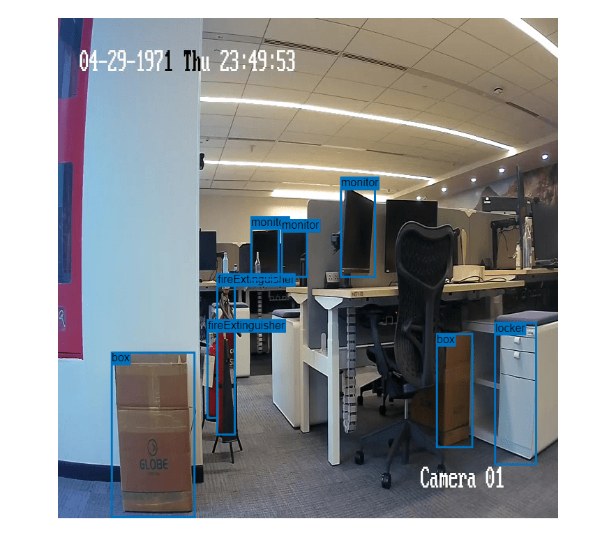
In this example, you label objects from four target classes: box, locker, monitor, and fireExtinguisher. You can use the datastore in the imageLabels.mat file attached with this example.

% Create the helper function.
function data = resizeImageAndLabel(data,targetSize)
% Resize the images and scale the corresponding bounding boxes.

    scale = (targetSize(1:2))./size(data{1},[1 2]);
    data{1} = imresize(data{1},targetSize(1:2));
    data{2} = bboxresize(data{2},scale);

    data{2} = floor(data{2});
    imageSize = targetSize(1:2);
    boxes = data{2};
    % Set boxes with negative values to the value 1.
    boxes(boxes <= 0) = 1;
    
    % Validate if bounding box in within image boundary.
    boxes(:,3) = min(boxes(:,3),imageSize(2)-boxes(:,1)-1);
    boxes(:,4) = min(boxes(:,4),imageSize(1)-boxes(:,2)-1);
    
    data{2} = boxes; 

end
officeLabelStruct = load('imageLabels.mat');
officeblds= officeLabelStruct.BBstore;

The size of all the images within the data set is [720 1024 3]. Based on the object analysis, the smallest objects are approximately 20-by-20 pixels.

To maintain a balance between accuracy and the computational cost of running the example, specify a size of [720 720 3]. This size ensures that resizing each image does not drastically affect the spatial resolution of objects in this data set. If you adapt this example for your own data set, you must change the training image size based on your data. Determining the optimal input size requires empirical analysis.

inputSize = [720 720 3];

Combine the image and bounding box datastores.

officeds = combine(imds,officeblds);

Use transform to apply a preprocessing function that resizes images and their corresponding bounding boxes. The function also sanitizes the bounding boxes to convert them to a valid shape.

preprocessedData = transform(officeds,@(data)resizeImageAndLabel(data,inputSize));

Display one of the preprocessed images and its bounding box labels to verify that the objects in the resized images have visible features.

officedata = preview(preprocessedData);
I = officedata{1};
bbox = officedata{2};
label = officedata{3};
imshow(I)
showShape("rectangle",bbox,Label=label);

Define YOLO v2 Object Detector Architecture

Configure a YOLO v2 object detector using these steps:

1. Choose a pretrained detector for transfer learning.

2. Choose a training image size.

3. Select which network features to use for predicting object locations and classes.

4. Estimate anchor boxes from the preprocessed data used to train the object detector.

Select a pretrained Tiny YOLO v2 detector for transfer learning. Tiny YOLO v2 is a lightweight network trained on COCO [1], a large object detection data set. Transfer learning using a pretrained object detector reduces training time compared to training a network from scratch. Alternatively, you can use the larger Darknet-19 YOLO v2 pretrained detector, but consider starting with a simpler network to establish a performance baseline before experimenting with a larger network. Using the Tiny or Darknet-19 YOLO v2 pretrained detector requires the Computer Vision Toolbox™ Model for YOLO v2 Object Detection support package. For more information see, yolov2ObjectDetector (Computer Vision Toolbox).

pretrainedDetector = yolov2ObjectDetector("tiny-yolov2-coco");

Next, choose the size of the training images for YOLO v2. When choosing the training image size, consider these size parameters:

1. The distribution of object sizes in the images, and the impact of resizing the images on the object sizes.

2. The computational resources required to batch process data at the selected size.

3. The minimum input size required by the network.

Determine the input size of the pretrained Tiny YOLO v2 network.

pretrainedDetector.Network.Layers(1).InputSize

ans = 1×3

   416   416     3

YOLO v2 is a single-scale detector because it uses features extracted from one network layer to predict the location and class of objects in the image. The feature extraction layer is an important hyperparameter for deep learning based object detectors. When selecting the feature extraction layer, choose a layer that outputs features at a spatial resolution that is suitable for the range of object sizes in the data set.

Most networks used in object detection spatially downsample features by powers of two as the data flows through the network. For example, starting from the specified input size, networks can have layers that produce feature maps downsampled spatially by 4x, 8x, 16x, and 32x. If object sizes in the data set are small (for example, less than 10-by-10 pixels), feature maps downsampled by 16x and 32x might not have sufficient spatial resolution to locate the objects precisely. Conversely, if the objects are large, feature maps downsampled by 4x or 8x might not encode enough global context for those objects.

For this data set, specify the "leaky_relu_5" layer of the Tiny YOLO v2 network, which outputs feature maps downsampled by 16x. This amount of downsampling is a good tradeoff between spatial resolution and the strength of the extracted features, as features extracted further down the network encode stronger image features at the cost of spatial resolution.

featureLayer = "leaky_relu_5";

You can use the analyzeNetwork (Deep Learning Toolbox) function to visualize the Tiny YOLO v2 network and determine the name of the layer that outputs features downsampled by 16x.

Next, use estimateAnchorBoxes (Computer Vision Toolbox) to estimate anchor boxes from the training data. Estimating anchor boxes from the preprocessed data enables you to get an estimate based on the selected training image size. You can use the procedure defined in the Estimate Anchor Boxes From Training Data (Computer Vision Toolbox) example to determine the number of anchor boxes suitable for the data set. Based on this procedure, four anchor boxes is a good tradeoff between computational cost and accuracy. As with any other hyperparameter, you must optimize the number of anchor boxes for your data using empirical analysis.

numAnchors = 4;
aboxes = estimateAnchorBoxes(preprocessedData,numAnchors);

Finally, configure the YOLO v2 network for transfer learning on four classes with the selected training image size and the estimated anchor boxes.

numClasses = 4;
pretrainedNet = pretrainedDetector.Network;
pretrainedNet = layerGraph(pretrainedNet);
lgraph = yolov2Layers(inputSize,numClasses,aboxes,pretrainedNet,featureLayer);

Initialize the random number generator with a seed of 0 using rng, and shuffle the data set for reproducibility using the shuffle function.

rng(0);
preprocessedData = shuffle(preprocessedData);

Split the data set into training, test, and validation subsets using the subset function.

trainingIdx = 1:70;
validationIdx = 71:85;
testIdx = 86:100;
dsTrain = subset(preprocessedData,trainingIdx);
dsVal = subset(preprocessedData,validationIdx);
dsTest = subset(preprocessedData,testIdx);

Data Augmentation

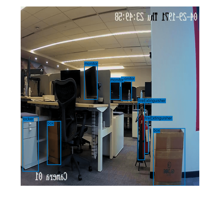
Use data augmentation to improve network accuracy by randomly transforming the original data during training. Data augmentation enables you to add more variety to the training data without increasing the number of labeled training samples. Use transform to augment the training data using these steps:

• Randomly flip the image and associated bounding box labels horizontally.

• Randomly scale the image and associated bounding box labels.

• Jitter the image color.

% Create the helper function.
function B = augmentData(A)
% Apply random horizontal flipping, random X/Y scaling, and jitter image color.
% The function clips boxes scaled outside the bounds if the overlap is above 0.25.
B = cell(size(A));

I = A{1};
sz = size(I);
if numel(sz)==3 && sz(3)==3
    I = jitterColorHSV(I, ...
        Contrast=0.2, ...
        Hue=0, ...
        Saturation=0.1, ...
        Brightness=0.2);
end

% Randomly flip and scale image.
tform = randomAffine2d(XReflection=true,Scale=[1 1.1]);  
rout = affineOutputView(sz,tform,BoundsStyle="CenterOutput");    
B{1} = imwarp(I,tform,OutputView=rout);

% Sanitize boxes if needed. This helper function is attached to the example as a
% supporting file. Open the example in MATLAB to use this function.
A{2} = helperSanitizeBoxes(A{2});
    
% Apply same transform to boxes.
[B{2},indices] = bboxwarp(A{2},tform,rout,OverlapThreshold=0.25);    
B{3} = A{3}(indices);
    
% Return original data only when all boxes have been removed by warping.
if isempty(indices)
    B = A;
end
end

augmentedTrainingData = transform(dsTrain,@augmentData);

Display one of the training images and box labels.

data = read(augmentedTrainingData);
I = data{1};
bbox = data{2};
label = data{3};
imshow(I)
showShape("rectangle",bbox,Label=label)

Train YOLOv2 Object Detector

Use trainingOptions to specify network training options.

opts = trainingOptions("rmsprop", ...
        InitialLearnRate=0.001, ...
        MiniBatchSize=8, ...
        MaxEpochs=20, ...
        LearnRateSchedule="piecewise", ...
        LearnRateDropPeriod=5, ...
        VerboseFrequency=30, ...
        L2Regularization=0.001, ...
        ValidationData=dsVal, ...
        ValidationFrequency=50, ...
        OutputNetwork="best-validation-loss");

These training options have been selected using Experiment Manager. For more information on using Experiment Manager for hyperparameter tuning, see Train Object Detectors in Experiment Manager (Computer Vision Toolbox).

To use the trainYOLOv2ObjectDetector (Computer Vision Toolbox) function to train a YOLO v2 object detector, set doTraining to true.

[detector,info] = trainYOLOv2ObjectDetector(augmentedTrainingData,lgraph,opts);

*************************************************************************
Training a YOLO v2 Object Detector for the following object classes:

* box
* locker
* fireExtinguisher
* monitor

Training on single CPU.
|======================================================================================================================|
|  Epoch  |  Iteration  |  Time Elapsed  |  Mini-batch  |  Validation  |  Mini-batch  |  Validation  |  Base Learning  |
|         |             |   (hh:mm:ss)   |     RMSE     |     RMSE     |     Loss     |     Loss     |      Rate       |
|======================================================================================================================|
|       1 |           1 |       00:00:04 |         8.01 |         5.91 |      64.2087 |      34.9198 |          0.0010 |
|       4 |          30 |       00:01:29 |         0.89 |              |       0.7946 |              |          0.0010 |
|       7 |          50 |       00:02:19 |         0.64 |         0.70 |       0.4086 |       0.4930 |          0.0001 |
|       8 |          60 |       00:02:44 |         0.55 |              |       0.3052 |              |          0.0001 |
|      12 |          90 |       00:03:55 |         0.45 |              |       0.2003 |              |      1.0000e-05 |
|      13 |         100 |       00:04:21 |         0.44 |         0.52 |       0.1956 |       0.2664 |      1.0000e-05 |
|      15 |         120 |       00:05:09 |         0.42 |              |       0.1766 |              |      1.0000e-05 |
|      19 |         150 |       00:06:21 |         0.41 |         0.50 |       0.1710 |       0.2478 |      1.0000e-06 |
|      20 |         160 |       00:06:46 |         0.44 |         0.49 |       0.1960 |       0.2447 |      1.0000e-06 |
|======================================================================================================================|
Training finished: Max epochs completed.
Detector training complete.
*************************************************************************

Detect Multiple Indoor Objects

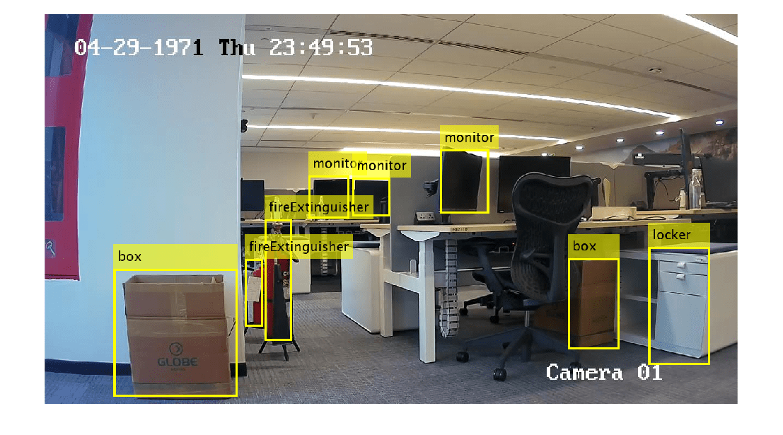
Read a test image that contains objects of the target classes, run the object detector on the image, and display an image annotated with the detection results.

I = imread(fullfile(datapath,"image_1.jpg"));
[bbox,score,label] = detect(detector,I);

annotatedImage = insertObjectAnnotation(I,"rectangle",bbox,label,LineWidth=4,FontSize=24);
figure
imshow(annotatedImage)

If you want to run object detector on the image captured directly from the IP Camera, run the following commands in the MATLAB Command Window.

for i=1:20
    img=snapshot(cam);
    [bbox,score,label] = detect(detector,I);
    annotatedImage = insertObjectAnnotation(I,"rectangle",bbox,label,LineWidth=4,FontSize=24);
    figure
    imshow(annotatedImage)
end

Evaluate Object Detector

Evaluate the trained object detector on test images to measure the performance. Computer Vision Toolbox™ provides an object detector evaluation function (evaluateObjectDetection (Computer Vision Toolbox)) to measure common metrics such as average precision and log-average miss rate. For this example, use the average precision (AP) metric to evaluate performance. The AP metric provides a single number that incorporates the ability of the detector to make correct classifications (precision) and the ability of the detector to find all relevant objects (recall).

Run the detector on the test data set. Set the detection threshold to a low value to detect as many objects as possible. A lower threshold helps you evaluate the detector's precision across the full range of recall values.

detectionThreshold = 0.01;
results = detect(detector,dsTest,MiniBatchSize=8,Threshold=detectionThreshold);

Calculate object detection metrics on the test set results with evaluateObjectDetection, which evaluates the detector at one or more intersection-over-union (IoU) thresholds. The IoU threshold defines the amount of overlap required between a predicted bounding box and a ground truth bounding box for the predicted bounding box to count as a true positive.

iouThresholds = [0.5 0.6 0.7 0.8 0.9];
metrics = evaluateObjectDetection(results,dsTest,iouThresholds);

List the overall class metrics, and inspect the mean average precision (mAP) to see how well the detector is performing.

metrics.ClassMetrics 

ans=4×5 table
                        NumObjects    APOverlapAvg         AP            Precision             Recall     
                        __________    ____________    ____________    ________________    ________________

    box                     30          0.83262       {5×1 double}    {5×9489  double}    {5×9489  double}
    locker                  15          0.86912       {5×1 double}    {5×1527  double}    {5×1527  double}
    fireExtinguisher        30          0.51511       {5×1 double}    {5×6037  double}    {5×6037  double}
    monitor                 45          0.75493       {5×1 double}    {5×11547 double}    {5×11547 double}

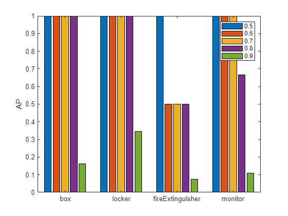
Compute the AP value at each of the specified overlap thresholds for all classes using the averagePrecision (Computer Vision Toolbox) object function. To visualize how the AP value at the specified thresholds values varies across all the classes in the data set, create a bar plot.

figure
classAP = averagePrecision(metrics);
bar(classAP)
xticklabels(metrics.ClassNames)
ylabel("AP")
legend(string(iouThresholds))

The plot demonstrates that the detector performed well on all the classes. If you are using your own image data set and see poor performance for certain classes, add more images that contain the underrepresented classes or replicate images with these classes, and then use data augmentation.

References

[1] Lin, Tsung-Yi, Michael Maire, Serge Belongie, Lubomir Bourdev, Ross Girshick, James Hays, Pietro Perona, Deva Ramanan, C. Lawrence Zitnick, and Piotr Dollár. “Microsoft COCO: Common Objects in Context,” May 1, 2014. https://arxiv.org/abs/1405.0312v3.

Related Topics

• Detect Circles from IP Camera Using Image Processing Toolbox
• Multiclass Object Detection Using YOLO v2 Deep Learning (Computer Vision Toolbox)