Output Function and Plot Function Syntax

What Are Output Functions and Plot Functions?

For examples of output functions and plot functions, see Output Functions for Optimization Toolbox and Plot Functions.

The OutputFcn option specifies one or more functions that an optimization function calls at each iteration. Typically, you might use an output function to plot points at each iteration or to display optimization quantities from the algorithm. Using an output function you can view, but not set, optimization quantities. You can also halt the execution of a solver according to conditions you set; see Structure of the Output Function or Plot Function.

Similarly, the PlotFcn option specifies one or more functions that an optimization function calls at each iteration, and can halt the solver. The difference between a plot function and an output function is twofold:

• Predefined plot functions exist for most solvers, enabling you to obtain typical plots easily.

• A plot function sends output to a window having Pause and Stop buttons, enabling you to halt the solver early without losing information.

Caution

intlinprog output functions and plot functions differ from those in other solvers. See intlinprog Output Function and Plot Function Syntax.

Note

Plot functions do not support the subplot statement, because the plot function framework manages the axes. To specify multiple subplots, write separate plot functions and pass them to the solver as a cell array:

options = optimoptions("solvername",PlotFcn={@plot1,@plot2,@plot3});

Output functions support subplot, so you can include multiple plots in one function by using an output function instead of a plot function.

To set up an output function or plot function, do the following:

1. Write the function as a function file or local function.

2. Use optimoptions to set the value of OutputFcn or PlotFcn to be a function handle, that is, the name of the function preceded by the @ sign. For example, if the output function is outfun.m, the command

    options = optimoptions(@solvername,OutputFcn=@outfun);

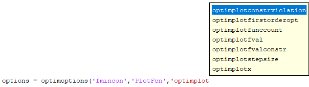
   specifies OutputFcn to be the handle to outfun. To specify more than one output function or plot function, use the syntax

    options = optimoptions(@solvername,OutputFcn={@outfun,@outfun2});

   To use tab-completion to help select a built-in plot function name, use quotes rather than a function handle.

   

3. Call the optimization function with options as an input argument.

Passing Extra Parameters explains how to pass parameters or data to your output function or plot function, if necessary.

Note

The optimplot plot function plots into a new window, not shared with any other plot function. For an example, see Monitor Solution Process with optimplot.

Structure of the Output Function or Plot Function

The function definition line of the output function or plot function has the following form:

stop = outfun(x,optimValues,state)

where

• x is the point computed by the algorithm at the current iteration.

• optimValues is a structure containing data from the current iteration. Fields in optimValues describes the structure in detail.

• state is the current state of the algorithm. States of the Algorithm lists the possible values.

• stop is a flag that is true or false depending on whether the optimization routine should stop (true) or continue (false). For details, see Stop Flag.

The optimization function passes the values of the input arguments to outfun at each iteration.

Fields in optimValues

The following table lists the fields of the optimValues structure. A particular optimization function returns values for only some of these fields. For each field, the Returned by Functions column of the table lists the functions that return the field.

Corresponding Output Arguments

Some of the fields of optimValues correspond to output arguments of the optimization function. After the final iteration of the optimization algorithm, the value of such a field equals the corresponding output argument. For example, optimValues.fval corresponds to the output argument fval. So, if you call fmincon with an output function and return fval, the final value of optimValues.fval equals fval. The Description column of the following table indicates the fields that have a corresponding output argument.

Command-Line Display

The values of some fields of optimValues are displayed at the command line when you call the optimization function with the Display field of options set to 'iter', as described in Iterative Display. For example, optimValues.fval is displayed in the f(x) column. The Command-Line Display column of the following table indicates the fields that you can display at the command line.

Some optimValues fields apply only to specific algorithms:

• AS — active-set

• D — trust-region-dogleg

• IP — interior-point

• LM — levenberg-marquardt

• Q — quasi-newton

• SQP — sqp

• TR — trust-region

• TRR — trust-region-reflective

Some optimValues fields exist in certain solvers or algorithms, but are always filled with empty or zero values, so are meaningless. These fields include:

• constrviolation for fminunc TR and fsolve TRR.

• procedure for fmincon TRR and SQP, and for fminunc.

optimValues Fields

OptimValues Field (optimValues.field)	Description	Returned by Functions	Command-Line Display
attainfactor	Attainment factor for multiobjective problem. For details, see Goal Attainment Method.	fgoalattain	None
cgiterations	Number of conjugate gradient iterations at current optimization iteration.	fmincon (IP, TRR), fminunc (TR), fsolve (TRR), lsqcurvefit (TRR), lsqnonlin (TRR)	CG-iterations See Iterative Display.
constrviolation	Maximum constraint violation.	fgoalattain, fmincon, fminimax, fseminf fminunc TR and fsolve TRR provide blank field values.	Max constraint or Feasibility See Iterative Display.
degenerate	Measure of degeneracy. A point is degenerate if: The partial derivative with respect to one of the variables is 0 at the point, and A bound constraint is active for that variable at the point. See Degeneracy.	fmincon (TRR), lsqcurvefit (TRR), lsqnonlin (TRR)	None
directionalderivative	Directional derivative in the search direction.	fgoalattain, fmincon (AS), fminimax, fminunc (Q), fseminf, fsolve (LM), lsqcurvefit (LM), lsqnonlin (LM)	Directional derivative See Iterative Display.
firstorderopt	First-order optimality (depends on algorithm). Final value equals optimization function output output.firstorderopt.	fgoalattain, fmincon, fminimax, fminunc, fseminf, fsolve, lsqcurvefit, lsqnonlin	First-order optimality See Iterative Display.
funccount	Cumulative number of function evaluations. Final value equals optimization function output output.funcCount.	fgoalattain, fminbnd, fmincon, fminimax, fminsearch, fminunc, fsolve, fzero, fseminf, lsqcurvefit, lsqnonlin	F-count or Func-count See Iterative Display.
fval	Function value at current point. Final value equals optimization function output fval. For fsolve, fval is the vector function value, and iterative display f(x) is the squared norm of this vector.	fgoalattain, fminbnd, fmincon, fminimax, fminsearch, fminunc, fseminf, fsolve, fzero	f(x) See Iterative Display.
gradient	Current gradient of objective function — either analytic gradient if you provide it or finite-differencing approximation. Final value equals optimization function output grad.	fgoalattain, fmincon, fminimax, fminunc, fseminf, fsolve, lsqcurvefit, lsqnonlin	None
iteration	Iteration number — starts at 0. Final value equals optimization function output output.iterations.	fgoalattain, fminbnd, fmincon, fminimax, fminsearch, fminunc, fsolve, fseminf, fzero, lsqcurvefit, lsqnonlin	Iteration See Iterative Display.
lambda	The Levenberg-Marquardt parameter, lambda, at the current iteration. See Levenberg-Marquardt Method.	fsolve (LM), lsqcurvefit (LM), lsqnonlin (LM)	Lambda
lssteplength	Actual step length divided by initially predicted step length	fmincon (AS, SQP), fminunc (Q)	Steplength or Line search steplength or Step-size See Iterative Display.
maxfval	Maximum function value	fminimax	None
positivedefinite	0 if algorithm detects negative curvature while computing Newton step. 1 otherwise.	fmincon (TRR), fminunc (TR), fsolve (TRR), lsqcurvefit (TRR), lsqnonlin (TRR)	None
procedure	Procedure messages.	fgoalattain, fminbnd, fmincon (AS), fminimax, fminsearch, fseminf, fzero fmincon TRR and SQP, and fminunc provide blank field values.	Procedure See Iterative Display.
ratio	Ratio of change in the objective function to change in the quadratic approximation.	fmincon (TRR), fminunc (TR), fsolve (TRR), lsqcurvefit (TRR), lsqnonlin (TRR)	None
residual	The residual vector.	lsqcurvefit, lsqnonlin,	Residual See Iterative Display.
resnorm	2-norm of the residual squared.	lsqcurvefit, lsqnonlin	Resnorm See Iterative Display.
searchdirection	Search direction.	fgoalattain, fmincon (AS, SQP), fminimax, fminunc (Q), fseminf, fsolve (LM), lsqcurvefit (LM), lsqnonlin (LM)	None
stepaccept	Status of the current trust-region step. Returns true if the current trust-region step was successful, and false if the trust-region step was unsuccessful.	fsolve (D)	None
stepsize	Current step size (displacement in x). Final value equals optimization function output output.stepsize.	fgoalattain, fmincon, fminimax, fminunc, fseminf, fsolve, lsqcurvefit, lsqnonlin	Step-size or Norm of Step See Iterative Display.
trustregionradius	Radius of trust region.	fmincon (IP, TRR), fminunc (TR), fsolve (D, TRR), lsqcurvefit (TRR), lsqnonlin (TRR)	Trust-region radius See Iterative Display.

Degeneracy

The value of the field degenerate, which measures the degeneracy of the current optimization point x, is defined as follows. First, define a vector r, of the same size as x, for which r(i) is the minimum distance from x(i) to the ith entries of the lower and upper bounds, lb and ub. That is,

r = min(abs(ub-x, x-lb))

Then the value of degenerate is the minimum entry of the vector r + abs(grad), where grad is the gradient of the objective function. The value of degenerate is 0 if there is an index i for which both of the following are true:

• grad(i) = 0

• x(i) equals the ith entry of either the lower or upper bound.

States of the Algorithm

The following table lists the possible values for state:

State	Description
'init'	The algorithm is in the initial state before the first iteration.
'interrupt'	The algorithm is in some computationally expensive part of the iteration. In this state, the output function can interrupt the current iteration of the optimization. At this time, the values of x and optimValues are the same as at the last call to the output function in which state=='iter'.
'iter'	The algorithm is at the end of an iteration.
'done'	The algorithm is in the final state after the last iteration.

The 'interrupt' state occurs only in the fmincon 'active-set' algorithm and the fgoalattain, fminimax, and fseminf solvers. There, the state can occur before a quadratic programming subproblem solution or a line search.

The following code illustrates how the output function might use the value of state to decide which tasks to perform at the current iteration:

switch state
    case 'iter'
          % Make updates to plot or guis as needed
    case 'interrupt'
          % Probably no action here. Check conditions to see  
          % whether optimization should quit.
    case 'init'
          % Setup for plots or guis
    case 'done'
          % Cleanup of plots, guis, or final plot
otherwise
end

Stop Flag

The output argument stop is a flag that is true or false. The flag tells the optimization function whether the optimization should stop (true) or continue (false). The following examples show typical ways to use the stop flag.

Stopping an Optimization Based on Data in optimValues

The output function or plot function can stop an optimization at any iteration based on the current data in optimValues. For example, the following code sets stop to true, stopping the optimization, when the size of the directional derivative is less than .01:

function stop = outfun(x,optimValues,state)
stop = false;
% Check whether directional derivative norm is less than .01.
if norm(optimValues.directionalderivative) < .01
    stop = true;
end 

Stopping an Optimization Based on GUI Input

If you design a GUI to perform optimizations, you can make the output function stop an optimization when a user clicks a Stop button on the GUI. The following code shows how to do this, assuming that the Stop button callback stores the value true in the optimstop field of a handles structure called hObject:

function stop = outfun(x,optimValues,state)
stop = false;
% Check if user has requested to stop the optimization.
stop = getappdata(hObject,'optimstop');