refcurve
Add reference curve to plot
Description
refcurve( adds a polynomial reference curve
to the current axes. The vector p)p contains the polynomial coefficients
in descending powers.
refcurve with no input arguments adds a reference line along the
x axis.
hline = refcurve(___)hline using any of the input arguments in the
previous syntaxes. Use hline to modify properties of a specific reference
line after you create it. For a list of properties, see Line Properties.
Examples
Generate data with a polynomial trend.
p = [1 -2 -1 0];
t = 0:0.1:3;
rng(0,"twister") % For reproducibility
y = polyval(p,t) + 0.5*randn(size(t));
Plot data and add the population mean function using refcurve.
plot(t,y,"ro")
h = refcurve(p);
h.Color = "r";
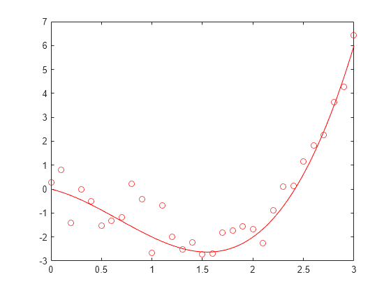
Also add the fitted mean function.
q = polyfit(t,y,3);
refcurve(q)
legend("Data","Population Mean","Fitted Mean",Location="NW")

Introduce the relevant physical constants.
M = 0.145;      % Mass (kg)
R = 0.0366;     % Radius (m)
A = pi*R^2;     % Area (m^2)
rho = 1.2;      % Density of air (kg/m^3)
C = 0.5;        % Drag coefficient
D = rho*C*A/2;  % Drag proportional to the square of the speed
g = 9.8;        % Acceleration due to gravity (m/s^2)
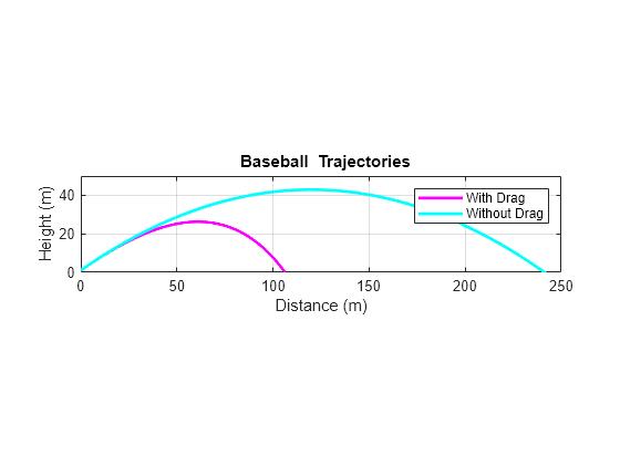
Simulate the trajectory with drag proportional to the square of the speed, assuming constant acceleration in each time interval.
dt = 1e-2;      % Simulation time interval (s)
r0 = [0 1];     % Initial position (m)
s0 = 50;        % Initial speed (m/s)
alpha0 = 35;    % Initial angle (deg)
v0 = s0*[cosd(alpha0) sind(alpha0)]; % Initial velocity (m/s)

r = r0;
v = v0;
trajectory = r0;
while r(2) > 0
    a = [0 -g] - (D/M)*norm(v)*v;
    v = v + a*dt;
    r = r + v*dt + (1/2)*a*(dt^2);
    trajectory = [trajectory;r];
end
Plot trajectory and use refcurve to add the drag-free parabolic trajectory (found analytically) to the plot of trajectory.
figure
plot(trajectory(:,1),trajectory(:,2),"m",LineWidth=2)
xlim([0,250])
h = refcurve([-g/(2*v0(1)^2),...
(g*r0(1)/v0(1)^2) + (v0(2)/v0(1)),...
(-g*r0(1)^2/(2*v0(1)^2)) - (v0(2)*r0(1)/v0(1)) + r0(2)]);
h.Color = "c";
h.LineWidth = 2;
axis equal
ylim([0,50])
grid on
xlabel("Distance (m)")
ylabel("Height (m)")
title("{\bf Baseball Trajectories}")
legend("With Drag","Without Drag")
Input Arguments
Output Arguments
Version History
Introduced before R2006a