Hardware-in-the-Loop (HIL) Testing of an Electric Motor Controller
Overview
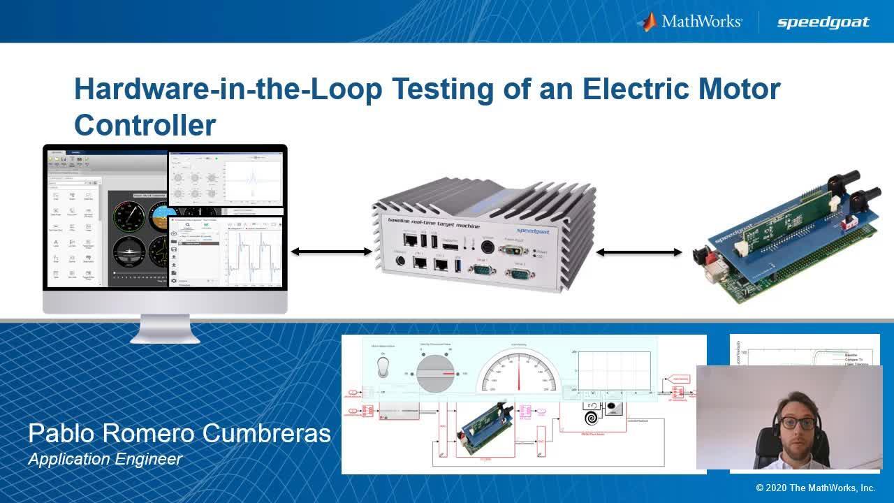
This webinar will demonstrate Hardware-in-the-Loop (HIL) testing of a controller for a 3-phase inverter and permanent magnetic synchronous motor (PMSM). A MathWorks engineer will show you how to run a motor and inverter model in real-time using Simulink Real-Time and a Speedgoat Real-Time Target Machine. You will learn how to configure your model for real-time testing, control your HIL application from within Simulink, create and manage test scenarios, verify and validate functional requirements, generate test reports, and automate your regression tests in the context of Continuous Integration.
Highlights
In this webinar, you will learn how to:
- Prepare a PMSM and inverter model developed using Simscape Electrical for HIL testing
- Control a HIL application from Simulink
- Test a microcontroller executing field-oriented control (FOC) algorithms developed with Motor Control Blockset
- Create and run test cases including execution instructions and assessments for the system under test using Simulink Test
- Manage your requirements and track their implementation and verification with your model using Requirements Toolbox
- Automate your testing and reporting, and integrate it to your Continuous Integration platform
About the Presenter
Pablo Romero Cumbreras is an Application Engineer at MathWorks specializing in real-time systems, verification, validation, and physical modelling. He previously worked at BMW Group modelling vehicle dynamics, and at Airbus Defence and Space validating flight control laws. He received his M.Sc. in aeronautical engineering from the Universidad Politécnica de Madrid and carried out his final project at the TU München.
Recorded: 24 Nov 2020
Hello, and welcome to this webinar on Hardware-in-the-Loop testing of an Electric Motor Controller. My name is Pablo Romero, and I am an application engineer at MathWorks. If you are currently working on an embedded software project, or have worked on that in the past, you may agree with me that converting that code that works and development computer to a final product requires multiple iterations and testing with many major milestone in between.
If you are leveraging model-based design for the development of your control system, you can use automatic production code generation to accelerate design iterations, and reduce the coding errors. Regardless of how you have achieved the implementation code, a long journey will start with thorough testing, sometimes involving certification processes to ensure and provide evidence that your system fulfills the technical requirements.
This testing process usually starts at component level, testing and verifying the code with software-in-the-loop. And upon completion and deployment to the final processor with processor-in-the-loop test. However, a later testing step is highly recommended to verify and validate the system functionality, including the interaction of different components, and the communication interfaces between them.
This can be achieved by performing hardware-in-the-loop testing, commonly known as HIL testing in the industry. HIL testing helps in catching errors before prototype testing, or product commissioning.
The goal of this webinar is to demonstrate how MathWorks and Speedgoat's real time testing solutions can help you to improve the quality and operational safety of your system. Verifying and providing evidence that the implementation code on embedded controller fulfills the technical design requirements to reduce risk and cost of in-field and prototype testing.
Using a permanent magnet synchronous model as an example, I will demonstrate how to transition from another stop simulation to real time testing, with the final controller board, and a Speedgoat real time target computer. You will learn how to run simulations in real time on the Speedgoat target for hardware-in-the-loop from Simulink.
You will see how to manage functional requirements, and trace their implementation and verification. Also, in a fully automated testing workflow to achieve their highest standards of quality accelerating the transition from software to hardware. In this webinar, we will not explain in detail the design and deployment of the control software.
If you want to learn more about this, we have some additional learning resources at the end of this webinar, including the prototyping of the field-oriented control algorithm used today on the same real time target computer hardware. Before diving in, please let me explain to this hardware setup.
We have a development, or host computer with MATLAB, Simulink, other design and code generation tools, and Simulink Real-Time, which is the product required for real time simulation from Simulink. Once we have deployed the control software to the controller board, or ECU, we'd like to reuse the plant model we have used for desktop simulation to perform Hardware-in-the-Loop testing.
We will generate code, and deploy this model to a Speedgoat target computer using Simulink's automatic code generation technology. The Speedgoat real time target computers with I/O models allows you to interface with your device and their test. For our sample, we are using a Speedgoat target computer with multi-core CPU, and an I/O model to interface BPM signals, and phase currents with embedded controller board.
This is the same Speedgoat target computer that my colleague Chirac used to prototype their motor control algorithm. However, in this case, we will reconfigure the Speedgoat's I/O module, and run our plant model in real time on the Speedgoat while the control runs on the final production hardware.
The HIL kit includes an embedded controller board a Speedgoat PCB to interface with the Speedgoat's I/O module, configured to capture the three phase parent signals as well as all the detail and analog lines, which are required for the complete setup. In the first section, you will learn how to prepare the PMSM and inverter plant model for real time simulation.
We model our complete system in Simulink to accelerate the design of the controller because it allows us to test different strategies and parameterization quickly. Besides, if we have a detailed plant model, we have a closed loop virtual test bench for more detailed simulation.
One of the advantages of model-based design is that we can reuse the plant model we have used on our development computer for real time testing on the Speedgoat hardware. Let's see how we can do it. This is the plant model we will use for today's webinar. We can see the permanent magnet synchronous machine model on the left, whereas on the right, we have emulated some motor sensors, such as the motor encoder.
Let's look at the PMSM plant model in more detail. We can see there are different possible variants. They provide different levels of fidelity, and may leverage other Simulink toolboxes. I will use this Simscape variant, because it offers the best way to model complex physical systems in Simulink.
You will work with circuit diagrams connecting different physical components of multiple domains, such the electrical and mechanical that are represented in blue and green colors, respectively. And those abstract from their detailed implementation of differential equations in the time domain from Simulink.
In this level, we see the inverter, the motor, as well as other additional components, and the server configuration for Simscape. We will come back to this topic later. For now, let's have a closer look at the motor model. We see the PMSM block, which we have taken data from the Simscape electrical library.
Our parameter size, according to the specification of the model that the hardware seller provides. As you may have seen in the prototyping webinar, which I will link at the end of this presentation, we can use measurements taken with the Speedgoat to obtain the missing parameters we need for a high fidelity plant model.
In the other subsystem, we find a three phase two level inverter. We won't go into detail about the different options for its implementation. I would just like to mention that we are using average reaching for the sake of simplicity for this webinar. For a more accurate simulation, and being able to simulate following scenarios of single switching devices, we can use the same model architecture and select in the dropdown menu any of the other options.
I have already set the parameters in the plant model accordingly. Now we can use it for our complete closed loop system simulation on desktop. We are now at the top level of our PMSM model for desktop simulation. On the left side, you see the field-oriented control implementation that we have developed in Simulink and Stateflow and that we have tuned with the prototyping on our Speedgoat baseline, as shown in the first webinar.
Therefore we can run a simulation I have already prepared with a double step speed command to validate our control and plant model in closed loop. We use the simulation data inspector to plot this simulation results. We see that the model responds to the velocity command as we expect, based on previous observations with the hardware prototype.
And we can use the plant model for the verification states in Hardware-in-the-Loop. We have used a variable step solver, which is the best trade-off between simulation and speed and accuracy for desktop. However, this software is not compatible for real time simulation because it is not deterministic.
For real time simulation, we must use a fixed-step solver. To set the solver and other configuration parameters required for real time simulation, we can use the Simulink real time button under the apps tab to configure our complete system in one single step. This operation also sets the system target file to Simulink Real Time.
Before deploying the plant model to the real time system, we should perform some simulations on the desktop to validate the solver, and sample time settings with the new results. For this purpose, I will use the same inputs as in the previous run, and compare the results using the simulation data inspector.
We can see that the result match very well. And therefore, our current settings meet the accuracy requirement. However, we have noticed that the simulation was slower than before, and might not be capable to run in real time on the hardware. One way of achieving faster simulations is increasing the sample time. But we may face some numeric inaccuracies.
Also, we may explicitly split our model into different tasks to balance the workload of the different codes on the Speedgoat CPU. However, our first option should be discretizing the Simscape plant. Continuous solvers are accurate, but are also computationally expensive.
And sometimes, if the sample time is small enough, they may not provide any major advantage. Discretizing the Simscape plant model is easy. We must just open the solver configuration block of this Simscape network, and enable the local solver. This will discretize the physical model automatically, and solve it with a backwards Euler solver, which is much faster.
In addition, we may set a fixed number of nonlinear iterations so that our task execution time in real time simulation is constrained. And we don't find unexpected CPU overloads caused by its low convergent numerical iterations. As we did with the fixed-step solver, we have to validate the new server configuration on the desktop.
We run the same test case again, and use the simulation data inspector to compare the results. They match the reference, because the sample time is small enough. We'll have a better performance in real time simulation and in desktop. So we may use the local solver as well in offline simulation to achieve faster runs while keeping the accuracy as I have just shown.
We have just seen how to model complex physical plants with Simscape for a closed loop simulation on desktop, how to configure this model to enable real time simulation and faster simulation thanks to the local software. After having successfully configured the PMSM and inverter plant models for real time simulation, in the next section, you will see how to do a Hardware-in-the-Loop simulation to test the embedded controller.
This diagram, we see our starting point. This represents the model that we have just used in desktop simulation. We can see the field-oriented controls subsystem on the left, and the PMSM plant model on the right, surrounded by the test suite where we define the inputs for the simulation and some verification functions.
This is just one example we have selected for this webinar. But you can replace this with a controller and plant models that may be more related to your current project. In a Hardware-in-the-Loop scenario, we have our embedded controller physically available and ready to be tested.
Previously, we have implemented the control algorithm on it, either by hand coding or by a more efficient and less error-prone automatic code generation. As we have the controller ready, we will replace its representation on the original model with the I/O driver blocks that will configure the I/O Speedgoat interfaces so that we can interact with them via the controller our device and their tests.
Coming back to our test scenario, we have their field-oriented control running on the controller board. The PMSM model, together with the I/O driver blocks, on the host computer, on a Speedgoat target computer where the real-time simulation will run. In just one click, we will generate code from the plant model, and other required components on the host, which will be compiled and linked to make a real time application.
This real time application is a container file that includes an executable for the real time operating system running on the Speedgoat. It will be transferred to it via ethernet, and thus, we will carry out the Hardware-in-the-Loop test. Let's see how this works in Simulink.
This is our PMSM model for HIL simulation. As you can see, it is very similar to the one we have used in the previous section. Actually, the plant model is essentially the same, because we are using a model reference and it is already configured for real time simulation. The main difference is that we have replaced their field-oriented control algorithm with the Speedgoat driver blocks that will allow the Speedgoat target to interact with the controller board.
Let's have a closer look at it. At this level, I have grouped separately the outputs and the inputs. First, we will inspect the Speedgoat outputs, which are the inputs for our device under test. As you can see, we have different blocks for the interfaces.
Starting from the top, this is the set up block for the configurable I/O module. As I commented earlier, with this block you can configure an FPA with different functionality so that the same I/O module carries out completely different task. This is possible thanks to multiple bit stream.
They are provided by Speedgoat according to our specifications. In my case, I can inspect the pin mapping, and check that mine includes the three PBM capture lines. A Quadrature encoder, SBI, and some general purpose digital lines. Here at the bottom, we see the analog pins available.
After setting the bit stream we will use, we just have to start adding and configuring the Speedgoat I/O driver blocks. We can download them from the Speedgoat customer portal, and upon installation, they will show up in the Simulink library browser as any other tool box.
We will find that blocks for all the I/O models available, which we can add to the model we are building. In our case, I have an interrupt block to capture the interrupt signal internally generated by the FPA so that I can synchronize the clocks of both the controller and Speedgoat CPU.
In addition, we have some detail outputs. The quadrature in color for the velocity feedback, and some more analog outputs for the closed loop. Please notice that the Speedgoat I/O models can be configured directly from the driver blocks as any other Simulink component.
Besides, every driver block has its own documentation completely integrated into MATLAB so that you can get all the information you may need to set it up. In the other subsystem, we have the outputs from embedded controller that are captured by the Speedgoat target computer.
The most important one is the PWM capture block. The pulse width modulation signal is sampled at a faster rate at the hardware level, and the most recent duty cycle value is provided at a specific model sample time. This three dimensional signal will feed directly the inverter block, because we are using the average reaching.
Let's go back to the top model level and proceed with the step we have been waiting for. After having validated our plant model in closed loop simulation on desktop, and having configured I/O driver blocks, it's time to test our embedded controller in real time. Using the real time menu, we select a target computer we'd like to use and connect to it.
Then we click on the run on target button that will take care, in one single action, of all the steps required to run this model in real time on the Speedgoat target computer. It will create the real time application, transfer it to the Speedgoat, and initiate external mode to control and monitor the real time simulation directly from within Simulink.
If desired, we can run this step separately by using the drop down menu below the run on target button. To control and monitor this simulation in real time, we will use the floating instrument panel that you may have already seen minimized in light blue. By double clicking on it, we can expand it, and use it to command the motor velocity when the real time simulation starts on the target.
We will see immediately signals being streamed to their host for live monitoring. Using the gauges and interrupts, we can control the application. In the same way, we could modify any block mask, or any parameter starting the workspace as we were simulating on desktop.
Instrument panels provide a user-friendly and visual way of interacting with the simulation. We see that the model reacts to our commands. Also, if we switch off the motor it goes down to zero, like this experiment we did in the prototyping. We can also switch it back on. Thus, we have easily performed a Hardware-in-the-Loop test of our motor control running in the embedded hardware, which receives high speed command, and commands a three phase pivot signal captured by the FPA on the Speedgoat.
The target computer also runs in real time the PMSM Simscape plant model we used in desktop providing the same results. Let's recap what we have just seen. The run on target button from this Simulink tool strip automates the transition from desktop to real time simulation.
It generates the code, and creates the real time application that they Speedgoat target computer executes. In this sample, we have used our PMSM as an inverter plant model that matched the Speedgoat model kit we used for prototyping. You may replace this representation with any other plant model that represents your final system.
We have also learned how the Speedgoat's configurable FPAs help us provide a flexible I/O interface for the hardware under test. Providing digital analog converters and vice versa, as well as capturing the PBM signal at a very fast rate to obtain the duty cycle we need for the plant model running on the CPU.
We may use the configurable I/O module for many other communications. Simply changing the configuration file that the Speedgoat provides according to the code modules, we can see on the screen. We have seen so far how to run Hardware-in-the-Loop test cases starting from a Simulink model that we set up for real time simulation on the Speedgoat target computer.
The previous section, you saw that we can perform HIL testing interactively directly from so Simulink model in a external mode. However in most of their real HIL scenarios, we would like to create many test cases to test the hardware in different situations, and automate the testing as much as possible so that we don't have to manually select, load, execute, and then evaluate the simulation runs.
In this section, we will see how the Simulink framework help us to achieve this goal. This automation should be considered from the first stages of development. We should create and automate testing as far as possible, including desktop simulation, or in other words, modeling the loop.
You can see this on the right diagram. The controller and plant models represent in Simulink our system under test. Separating test definition and evaluation from the system under test, these have us practice for efficient testing.
We can encapsulate it in test harness, which is a single functional entity with the input and output interfaces so that we can define and connect multiple test inputs and verification statements separately and independently from the model we are testing.
This gives us the flexibility so that model development and creation of test cases are managed in parallel thanks to the common interfaces that this harness provides. A great advantage of this workflow is that we can replace any part of the model or system under test with a real, physical component to perform Hardware-in-the-Loop simulation.
This is the most efficient and flexible way for testing and achieving a consistent workflow from desktop to real time. Because we will reuse the same test configuration and cases we had used for model-in-the-loop for Hardware-in-the-Loop saving much test development time, and ensuring traceability and consistency for the test at every step of the verification phase.
Let's see how we can do it with a real example. We will start with our PMSM system model. At the beginning of this presentation, we use a signal builder to define the inputs of our model. This is a quick way of testing, but has the drawback of modifying this system under test for every little change.
We can use test harnesses as we have just seen to separate the definition of test cases and the model we are testing. First of all, I will switch the active variant to harness to enable the top model input ports you can see on the left. This provides no functionality, but simply connecting both sides of the input variant subsystem.
The test harness will use the ports of the component to test. We may create test harnesses for every component of our system to perform unit tests, or create them for complete models. In any case, you use the right click to create a test harness for the system to test.
In this example, we have already available some test harnesses. As we were focused on plant modeling, our colleague in charge of testing used the top model ports we agreed to create some test harnesses. Now, we'd like to try them. We can switch to a test harness using the perspective use icon on the bottom right corner of the model window.
It will open different perspectives, including code and requirements, and display a view of every test harness for the current model. We want to test the one that uses a test sequence block. You can see that this harness looks like as any than model, but it includes automatically the system and their test as a model reference as it were a test page.
We don't have to worry about what's inside, but use the model interface to define the test inputs and verification we need. In this test harness, we have used a test sequence block to define on one single place the inputs and verification for the test case. We will find multiple steps in the test sequence editor to define the commands for our model.
The conditions to enable a step transition and thus achieve closed loop testing, as well as additional columns to set the sequence order, and provide further information. In this example, we start the test gate at zero and with the motor off. After one second, we start the motor.
It will go through some encoder calibration, and eventually reach the closed loop state. We wait for one second during this step before commanding a positive velocity step, and wait a certain set of time that we have defined as a parameter to verify that the velocity response of the motor, less within tolerance. We will repeat the process with a velocity command in the opposite direction.
And finally, set the model to still stand. We can run this test case on desktop, and inspect the results as we did earlier. During the execution, we see highlighted in blue the current state. And eventually, add break points to debug the execution of the test sequence. We use the simulation data inspector to plot the velocity signals, and to check the verification results we have included to verify the response tolerance to a step command.
We see that all checks are passed, and therefore that this case was successful. We have run the test sequence in model-in-the-loop, but as commented before, we want to reuse test cases for real time simulation, too. In this case, what we can do is link in the test sequence block to a test harness for our PMSM HIL model. As you can see, the test harness looks the same.
We could use the run on target button to immediately execute it in real time on this bigger target computer. However, we may end up with a lot of different model and test harnesses. And we have said our intention was to avoid managing them manually. To ease and unify their management, execution, and inspection of all type of test cases, we will use the Simulink test manager.
In the Simulink tool strip, we see the harness tab that collects the most relevant comments for testing. On the right side, we see the bottom to open the test manager. On the new dropdown menu, you see the different options to start working on our test strips. We may start with a block test file, and add some of the best cases we find available, such as their baseline, simulation, equivalence, and real time test cases.
If we liked some help, we can use one of the options below to get an assistant to create test cases automatically based on some assisted models or files. For today's example, I will open one assistant test file in our Simulink project. This test file contains different folders and test cases.
We can create an ordered hierarchy as we need. Later, we can decide if we want to run single test cases, suites, or the complete test set up. As we did at the beginning of this section, we'll start with the model-in-the-loop test case. This simulation test, used the desktop model and test harness we saw earlier.
We won't have to open it manually to execute it, but use the test manager to manage it completely. On this page, you will see different options to configure the test, according to your test specifications. We have just commented how to set up the model or system under test. You may override the simulation settings, or use the default ones set at the model.
The parameter override section is very helpful to automate the testing of different parameter sets. Instead of creating our own test script of different copies of the same model, we can use it to define different parameters that will be calculated with the model set above. Please notice that in this case, we will override the physical value of our plant model, the inertia of the spinning disk.
We will thus validate if our control can handle well different values, ensuring our velocity responds within the tolerance limits defined in the test sequence block. Please notice that in this test case, we will override our physical value of our plant model, the inertia of the spinning disk.
We will thus validate if our control can't handle well different values ensuring our velocity response within the tolerance limit defined in the test sequence block. In addition, we may use the following sections to configure additional callbacks, inputs that may not be defined in the test harnesses, or the output we'd like to land on top of the locked signals in the model.
We will use the configuration above to create the iterations, or runs, we want to execute. And finally, we can define some logical, temporal, or custom assessments to validate the requirements, as we'll see in the next webinar section. For now, let's run this test case. We see that there is a total of three test runs for every parameter set.
They are executed sequentially, but we could parallelize the execution of these test cases by simply enabling the parallel button in the tool strip. Results will be presented for every iteration. We can inspect them manually as we did with the first stop simulation in the data inspector. And effectively, verify that the increment in the inertia causes a low error response of the model.
And still the controller is able to respond as suspected, and the verification statements are fulfilled as we can see in the status column on the left. We will continue the controller testing with the Hardware-in-the-Loop To do so, we don't have to create another test case from scratch, but we can convert to the last one to a real time test case from the context menu.
The real time test case, which I have renamed to HIL, will execute this simulation in real time on the Speedgoat target computer, connecting to it, and building the real time application as we did earlier, if required. As you can see, we are using the parameters, callbacks, assessments, and other configurations that we have defined previously.
For the sake of convenience, we have selected the appearance and HIL model instead, because it's the one containing the I/O driver blocks. We will execute the same scenario, but this time on the real time target. The test manager is now building the real time application.
This will take some time, but later iterations will be immediate, because changing parameters doesn't require a model rebuild. We may select to use one assistant in real time application already built on the host. Or on the target, if available. And escape, therefor, the initial builder step. We get the results ready to inspect as soon as the target has completed every iteration.
We see that the results are similar to the ones obtained from desktop simulation, and that the embedded controller has passed the test after all the verification assessments have been automatically verified. In this case, we have executed the model-in-the-loop and the Hardware-in-the-Loop test cases separately.
We could run the complete suite, and the test manager will run every test case on its corresponding platform. In addition, we may run some equivalent test cases to ensure that tests on desktop and on Speedgoat match considering certain equivalence criteria.
Once we have a complete set of results, we may want to export them for a later analysis, or documentation. Or create a test reported so that results are quicker to consult. For example, we wouldn't need to open the test manager but just read an ordinary PDF report that was automatically generated.
We can select the test cases we want to generate the test for, and click on the report button. Please notice we can not only create a report for the results, but also for the test specifications. Today, we will focus on the results report. You can see that there are multiple fields we can customize, and check boxes to enable which content we want to publish.
There are several formats available. PDF, a word document, or zipped file with HTML documentation. I will leave the standard configuration, and create a PDF report of the results we have just executed. We are currently triggering manually the creation of the test report. But if defining the main test file, the report could be also generated automatically after the test execution with the specified content.
This is very useful for its integration in a continuous integration workflow as we will see later. In the meanwhile, the report is ready, and we see that all the results are available in an open PDF format. We can store it, or distribute it among other colleagues that don't have Simulink, but they still want to consult the results of the test automation.
Let's recap what we have just seen. We can use Simulink to design, run, and report test cases from model in the loop up to complete system level Hardware-in-the-Loop tests. The test manager is the main tool to create, manage, and monitor all the test cases, including those that run in real time on a Speedgoat target hardware, either for prototyping, or HIL testing.
We can classify test cases in different test suites, and enable or run then separate, or in groups. There are also controls for the normal test execution for debugging or for parallelizing in one single button those tests that should run on the development computer. Testing evolution results are collected and displayed in one common tool.
We have a summary of the pass fail criteria, and some text feedback. We can inspect their results in detail and create the reports in different format for distribution, or further reference. In the previous section, we have seen how to manage, execute, and report tests for our design.
However, unless you are doing this for a webinar, these test cases are not arbitrary , and your goal is to verify certain specifications according to the same requirements. In this section, you will see how you can offer, manage, and trace the same requirements within Simulink. You can track their status, and link them to their implementation in the models, as well as its verifications to the test cases we have created as shown earlier.
The reports that we will generate from them will provide traceability from requirements to code, and evidence that all requirements are implemented and verified. Let's look at a refresh sample in this moment. You may have noticed that in the header of every test case, there is a section called requirements.
This will allow us to link a requirement and a test case. In addition, to achieve better granularity, and a more direct connection between the requirement definition index and it's verification, we may create additional logic and temporal assessments that we can link separately to any requirement as shown in the column on the right. And those, we will verify multiple of them in one single test case.
There is a bidirectional traceability between our requirement and its verification. So we can click on every link to jump to the requirements editor where we will find all the requirements, definition, and implementation, and verification status. For the sake of time, I won't go much into detail about the editor.
But here, you have the option to define advanced properties and relationships for requirements. This example, we will consider a small set of requirements and its traceability status. At a first glance, you can see two columns that represent the current implementation and verification and status respectively. The third major requirement is just not linked to an implementation, as we can deduce due to its empty bar.
There are several ways to link requirements. One option is opening the implementation model and its requirement view from the bottom right corner. We will see which requirements are now open, and we may select them to highlight the active ones. To link our requirement to its implementation, we may use the context menu on the component we'd like to link, or select a requirement and drag it to its destination.
Immediately, a new link will appear on its property view, and the requirements editor will update the corresponding status. Moving on to verification, we can see that all off them have a full yellow verification column. If we hover with a mouse, we can see more details, meaning that all of them are linked, but not executed yet. We may select one of them, and check how they are verified.
Please notice that one requirement may be verified at different stages, starting from model-in-the-loop up to Hardware-in-the-Loop. Thanks to the bidirectional link, we will open the test case so that we can execute it and check its fulfillment. We can see that the test has passed, and its status has been, as well, updated.
As we have commented earlier, the test results report will include the verification of the requirements, but we can also create a requirements report directly from the editor for a more detailed documentation. Also MATLAB release 2020b includes a testing dashboard where you will get test snapshots to assess the quality of your requirement-based testing.
Let's recap how you can improve the quality of your design by managing and tracing your requirements to design, code, and test. You can use similar requirements to author and import textual requirements. Link requirements to the model Implementation in a few clicks. Create and link test cases for verification, and continuously monitor assess, and report quality with the requirement editor on the model testing dashboard.
We have seen up to now how to set up and execute a requirement-based quality testing, including Hardware-in-the-Loop tests on real time target computers. However, in a real scenario, we'd like to go one step farther so that we don't have to care about the test execution or reports. But only increasing the quality and functionality of our product.
We have done all that work preparing the model to run in real time, setting up the I/O interfaces. Even we have created a test environment that verifies our requirements. Why should we care when to run all these test jobs? Why not let an automation server execute everything we have created whenever necessary?
For example, a night when the system is not used to maximal efficiency, and therefore our investment in hardware. So that we have yet to consult the results of the validation criteria, and figure out when we need to fix something. Model-based design is a great workflow to allow engineers to implement and test ideas in simulation that they can later deploy on hardware.
And when mapped to a continuous integration workflow, we can be agile and iterate our design faster while delivering better products. Before submitting a change, we can simulate, test, and improve the design locally. This part of their workflow is what we have seen so far. Once we are satisfied with the results, and those may have passed some test, we can commit and submit the change to the repository.
When using a continuous integration workflow, every change pushed to the repository will trigger a reversion test, or a testing pipeline which will carry out some tests automatically, and may generate and publish some reports and other artifacts. And even deploy a new release version of their software. This ideal workflow is not exclusive of code, and can be used as well with MATLAB and Simulink together with the test suite requirements verification and report generation we have seen in this webinar.
This example, I will use Jenkins as an example of automation server with the MATLAB plugin for Jenkins to automate the execution of tests that I have previously created in Simulink tests. And also some made it to the repository in GitLab.
The corresponding results will be collected and published in Jenkins, and their build status will be reported back to GitLab. You can see in a sample of a job in Jenkins for a Simulink project. If we have a closer look at its configuration, we'll see that thanks to the MATLAB plugin for Jenkins, we can easily execute MATLAB functions and scripts containing the project.
And even automatically detect and run test files that we have generated with Simulink test. In addition from the job configuration, we can set the artifacts that we want to create. Please notice this is just an example with Jenkins. And this workflow is also reproducible with other automation servers. Either when executing their job on a regular basis, or upon a change detected in the repository, Jenkins will start at a MATLAB instance on a remote computer and run their cases according to our configuration.
We may add steps to collect and publish all kind of reports generated by MATLAB, including those PDF or HTML reports that we have generated with the test results so that we can store and consult them online. The test anything protocol planning integrated into MATLAB will also generate compact test results that are parsed by Jenkins for a quick results overview.
These results solve the project health trend and contain error log outputs from the MATLAB console. Depending on our continuous integration set up, we may even publish the status back to GitLab so that we can have our a directional link and life monitoring of MATLAB project.
Let's review the steps taken to leverage model-based design in a continuous integration workflow. We start locally on the development computer, creating the test cases and testing locally the design. In case we detect a failure, or we develop further the design, we do it locally and test it before submitting the changes with a detailed comment to the repository.
This will trigger a built-in automation server, for example, Jenkins, that will execute the test and verify the model, eventually collecting and publishing all the generated reports and artifacts. We started this webinar with a goal in mind. Let's wrap up today's presentation reviewing how we have achieved it.
We have presented a solution to improve the overall quality and safety of your system thanks to automating and extensive testing from model to Hardware-in-the-Loop That will help us to identify design flaws as early as possible. Thanks to their flexibility of model-based design, we can quickly design, implement, and verify changes that fulfill their technical design requirements.
And thus with reduced risk and cost to doing their verification and validation stage of embedded controllers with an agile workflow by reuse and testing of models from a desktop simulation to real time in a hardware-in-the-loop set up, either locally, or in automation servers. If you'd like to know more about the official real time solution from MathWorks together with the target computers designed and built by Speedgoat please take out these resources.
You will find learning material and trainings to help you ramp up quicker testing your models in real time. Also leveraging FPAs for high sample rates. If you are an engineer in the area of motor design or power electronics, please have a look at these webinars that complete the workflow shown in today's webinar with prototyping and further testing on FPAs.
Last, but not least, for those who specialize in HIL for battery management system, we have as well some recent and very useful learning resources. With this last recommendation, I conclude today's webinar about Hardware-in-the-Loop testing of an electric motor controller.
I hope you have enjoyed and learned a few things that are useful to test your embedded controller more efficiently in real time with a Speedgoat and Simulink in real time. Thank you very much for attending the webinar, and I wish you all a nice day.