Mixed-Signal Analyzer part 4: Working outside the app

Hello, this is Kerry Schutz with MathWorks. And this is part 4 in my video series on using Mixed-Signal Analyzer to post-process cadence simulation data. In this version, we're going to focus on automation and how to access the raw simulation data outside of Mixed-Signal Analyzer, so in base MATLAB. So, the functions that we'll cover today involve things that we've already shown in some previous videos on Mixed-Signal Analyzer. We'll just go into a little more detail this time around.

We're going to cover using adeinfo2msa and how to use it to save simulation data to a .mat file. We'll talk about a function that's msaSessionUpdate that you use to automate report generation. And we're going to be using those functions within cadence Maestro itself in the Output Setup section, as we'll see. And then, once we save the data to a .mat file, we're going to show how you can work with that raw data in base MATLAB, as opposed to using it inside the Mixed-Signal Analyzer app.

OK, so, let's go ahead and jump over into Cadence. And then, we'll go back into MATLAB. OK, so, now, we're back over in Cadence. We can see our Maestro setup. We've got different analysis types enabled, different design variables and global variables. This is our same LDL circuit that we were using in the other videos on Mixed-Signal Analyzer. We've got 20 corners, two point sweeps, and a nominal corner. And then, we've got our output setup.

And I covered this briefly in the previous videos. But we're going to go in a little more detail here. This is really the heart of the automation. The two MATLAB expressions or two MATLAB functions, we're calling here. OK, so, here, we're now over in Cadence again. We're inside of Virtuoso, got the Maestro view up. And we've got our same LDO circuit as before, same analysis type, same number of corners, et cetera. We've got 20 corners, two point sweeps, and a nominal corner for this.

And then, we have our output setup, which is really the heart of the automation that I want to cover here today. So, I'm going to go ahead and zoom in on that. So we can see it a little better. We've got two MATLAB expressions entered. And I'll just cover here the first one, the first one called adeinfo2msa. This function is going to open up a headless version of MATLAB upon conclusion of the simulation.

It's going to call this function, apply it to the adeinfo object that's in the base MATLAB workspace. And then, it's going to save both the metrics data and the waveform data to a .mat file. Now, in this case, that .mat, it's going to be auto-named based on the name of the test and the time date stamp. You could also optionally specify a file name. I'm just using the auto-naming convention here for convenience.

The other automation command, which you could run as well, although, typically, you would only run one of these commands. You wouldn't run both-- is MSA Session Update. So, instead of just saving the data to a .mat file and saying, we're done with it, it's going to go the extra step. And it'll take that data and apply some analysis to it. The analysis that's applied is saved in some session, in some mat file.

In this case, I'm just calling it, generically, session.mat. But it's whatever session file name you have specified here. The assumption here is that you've used Mixed-Signal Analyzer previously. You have manually performed some analyzes and visualizations on a data set. And then, you save that session file. And now, you're going to apply that to future data sets.

So, if we had that checked here instead, when the simulation was complete, it would take the new data set, apply this analysis that's specified in session.mat to it. It would create a report where, again, in this case, I didn't specify the report name. So, it's just going to use an auto-naming convention again with a time and date stamp on it. And it's going to save that in your Maestro's document folder by default, unless you specify a different path.

So, that's really the automation that I wanted to make sure everyone was aware of because, again, the whole idea here is that you don't have to manually open up MATLAB after each and every run. In Cadence, you can just automatically have either the .mat file saved. Or you can go ahead and generate a PDF PowerPoint, a file, as soon as the simulation is complete.

So, let's talk a little bit more about that data that gets saved when you call adeinfo2msa. What you're going to find in your MATLAB workspace is, again, you're going to find a .mat file and then a folder with a very, very similar name, for instance, the name of the test, the name of the interactive run. That would be the name of the folder, and then the name of the test and the name of the interactive run .mat file. You're going to find that pair.

You're going to find a folder file name pair associated with each and every adeinfo2msa save operation. And if you were to dig inside of the particular folders, you're going to find, subsequently, more .mat files that contain different types of your analyses. So, let's go into that a little bit more. Again, there are different variants of the adeinfo2msa command. We're not going to cover all those here.

I just wanted to show you how you could, for example, if you didn't want to use the auto-naming convention for the output file name, you could specify a file name argument and just type in whatever file name you wanted there, same with msaSessionUpdate. There are many options you can specify. I kind of used the bare bones version of msaSessionUpdate in my ade output setup that I showed earlier, something like you see here at the bottom.

OK, so, once we get that data into MATLAB, how can we work with it? So, again, after you save the data using adeinfo2msa, you're going to have a directory and a .mat file essentially by the same name, ldo_test, the name of your cadence test and the interactive run number, and then the folder, and then the .mat file. The directory here, let's just say it's ldo_test_interactive.2 that's going to hold waveform data. And then, the .mat file, let's say ldo_test_interactive.2.mat, that's going to have your metric data.

And then, if you look underneath at the waveform data folder, you're going to find more .mat files. And the reason you're going to find more .mat files is because, depending on the different types of analysis you had, you'll have one .mat file per node, per analysis type. So, in this case, I loaded ldo_test_interactive.3.mat. Within that .mat file, there's going to be two variables, file list and generic genericDB.

For the purpose of waveform data, you want to look at file list. It's kind of like your key to accessing the data that's in the waveform folder. It's going to say, hey, if you go to this directory and this file, you're going to grab the ldo out data for dc analysis. And if you go to this 1.2.mat in that same folder, you're going to get the transient for that LDL out node.

And again, that particular example that I have here just had two analysis types and one node in the circuit that I'd logged. Of course, you might have logged mini nodes and mini analysis types, in which case you're going to have, again, for each node, you're going to have the analysis that you've done on it. So, here, I've got three nodes. I've got two analysis types. So, it's three times two for the number of math files, which you're going to find in that file list folder.

OK, this follows. Again, so, 1.1.mat will have a dc simulation results. 1.2.mat will have dc simulation results for a different node, o1, and so on, 1.3.mat. We'll have dc simulation results for o2, and then the next three for the transient simulations. OK, so, again, here would be a sample session where we could access the data. It's assumed here that you've already done this save. Perhaps you've already called adeinfo2msa inside of your output setup of Cadence in the Output Setup section.

And now, over in MATLAB, you're accessing this data. Again, it could be on Windows, could be on Linux. You're going to load one of those. You're going to load the .mat file. And that .mat file is going to tell you what's in the waveform data folder. In this case, I've got the two analysis types and one node logged. So, now, I can see that directory with the waveform data. I can load 1.2.mat as an example, transient ldo_out. I can grab the x-axis values, the y-axis values.

And these are, again, variables within 1.2.mat. And then, I can plot them out. So, in this case, I just plotted corner 1 of so many corners, just an xy plot because x here is time. y just happens to be voltage in this case. And I can just plot that out, like anything else in MATLAB. So, next, let's go over to MATLAB and actually run this script.

So, I'll minimize PowerPoint. We'll go over to MATLAB. And what you're going to see is, I have that very, very same .mat file folder combination. So, what I'm going to do is, I'll just clear everything out, clear my screen. We will load. I'm just going to do what I showed you, ldo_test_interactive3.mat. You're going to see, I have two variables, filelist and genericDB. For the waveform data, I want to concentrate on filelist. For the metrics data, it's in GenericDB.

So, let's just type out filelist. And you'll see, if I make that bigger, it's going to make all that wider. You can see which file has what data in it under ldo_task_interactive3, under that folder. So, we will go underneath Interactive_3. And I have a little script which I put in there, conveniently, the same as I showed you in the PowerPoint for processing the data in 1.2.mat, in this case.

So, if I open up that script, you're going to see that I am here I'm loading 1.2.mat with the transient ldo_out data. I'm grabbing certain values. And then, I'm plotting them. So, if I do that manually, I could go over here. I could say-- I no longer need what I have there. So, I'm going to clear all my variables out so you can see more clearly what's in these .mat files. I'm going to load 1.2.mat.

You're going to see that it has wave names, x-axis labels, units and values. It's the values that are most interesting that has the time samples in x and the voltage samples in y-axis values. And then, you're off to the races in the script. If you just want to look at the first corner, just index by one. And that's what I did.

In this case, if you wanted to plot all of the cases, you could certainly just have a loop which goes from one to the number of cases, the length of x, where x is the length of x, x values. And you could plot all of them out. So, if I just run that portion, we could do that, evaluate that. You get that plot. Now, that's plot, of course, generated with my script. But if we were to go over to Mixed-Signal Analyzer and plot ldo_out, you'd get the very same plot, except here, it's in the inside of the Mixed-Signal Analyzer app.

And then, there's all kinds of things now you can do once you have the raw data in MATLAB. One thing I did here was, I wanted to re-sample the data. But I wasn't sure at what rate. So, what I did was, I took the time samples. And then, I computed the mean and the instantaneous sample rate. So, if I run this section of code and just plot it up to here, let's see. Did I do that right? Let's see.

Let's go ahead and run it. I'll run it all the way to right here. OK, so, this should plot out here the sample rate. As we are sampling that ldo_out signal, it's a variable step, Solver, our simulation engine. So, you're going to see that the sample rate is changing up here from about 1e9 up at the fast side. Down here, it's less than 1e8. And then, the mean sample rate is the one you see here in red, where the instantaneous is in blue.

So, that gives me some idea, if I'm going to do some re-sampling operation on this signal, what sample rate I should choose. And that's what I did in this script right here. And it ended up, I decided on about 1e9 to use. I re-sampled at that rate. And then, I did some spectral processing in this section right here. You just evaluate that. Here, you see the spectrum of that signal.

So, again, once you're in MATLAB, there's nothing you really can't do. This was another example where I continued to use the MATLAB slew rate function to compute the slew rate for corner one. So, again, I'm using the voltage data and the time samples. And plot out this slew rate. All right, so, that's good enough probably on the waveform side of things, how you can post-process it.

Next, let's focus on the metrics data. OK, the next capability I want to talk about is how to access the metrics data. And one thing to keep in mind for everything when it comes to, whether it's accessing waveform data or metrics data, is that what I'm showing you here is essentially an undocumented capability. In the future, it may become a documented capability. But at the present, in our 2023b, it is not.

The intent is to work through the Mixed-Signal Analyzer app in order to access and visualize, process the data. But I'm kind of showing you some backdoor techniques here in this video, in case you'll need to do something that the app doesn't support. And waveform data and metrics data access are two of those things. So, and what you'll notice about metrics data in particular is that it's a little bit more involved than accessing waveform data.

And the reason for that is when you're working with metrics data, you could be computing anything. With waveform data, you only have volts versus time or current versus time, something relatively simple, maybe power versus time. With metrics data, you could be computing any arbitrary quantity. It could be a phase margin, as we all have here, a slew rate, rise time. It could be computing delay, settling time, lock time, if it's a PLL overshoot, just anything.

With metrics, there's no limit to what you could compute. And also, of course, you are computing these metrics across many corners. And so, the result of that is, when we look at the data and how it's stored, you're going to see a lot more variables, a lot more fields. All right, so, let's just jump into an example. Using our previous ldo example, I'm loading the .mat file, the same .mat file we loaded, that we had created, and we had loaded before.

OK, so, for instance, if I go maybe back a page, if I go back a page, remember, we had our ldo_test_interactive.3, or .2, whichever one you had. That's the folder with the waveform data stored. But now, we're going to concentrate on this ldo_test, either .2 or .3.mat. These are where the metrics are stored.

OK, and so, we're going to load one of those files, in this case, .3.mat. And what you'll find is there's two variables stored in those files. There's a file list that's for accessing the waveform data. And there's GenericDB for accessing the metrics data. And both of these variables, you can think of them like keys. They're keys which tell you about the data. So, filelist didn't hold the waveform data. It told you where the waveform data was stored.

GenericDB also has that capability. It actually does both. It tells you something about the data. But it also holds the data itself. So, it's kind of a one stop shop in that sense. So, the first thing we're going to do with GenericDB is we're going to pull out field simulation results objects of 1. It's just a unit length cell array. I'm going to save that for a short name here, sro, simulation results objects.

Within simulation results objects, there's a few fields. Well, there's more than two. But there's two I'm going to say of interest primarily. One is called ParamNames. And one is called ParamValues. So, I just save those to PN and PV for short. And if you look over here, you'll see what is included in those. There are cell arrays. And in my case, it was a 22 by 1. But that length will be a function of your particular configuration test setup and cadence.

In my case, I had five variables that I was sweeping or changing over the course of my simulation, a load current, a capacitor value, process corner, temperature and voltage. Of course, you could have more than that. And then, that's in the process. And that's in the parameter names. For ParamValues, they're the corresponding values. So, what was that particular current value? What was that particular capacitor value, et cetera, associated with those parameter names? And that's what the parameter value cell array is going to tell you.

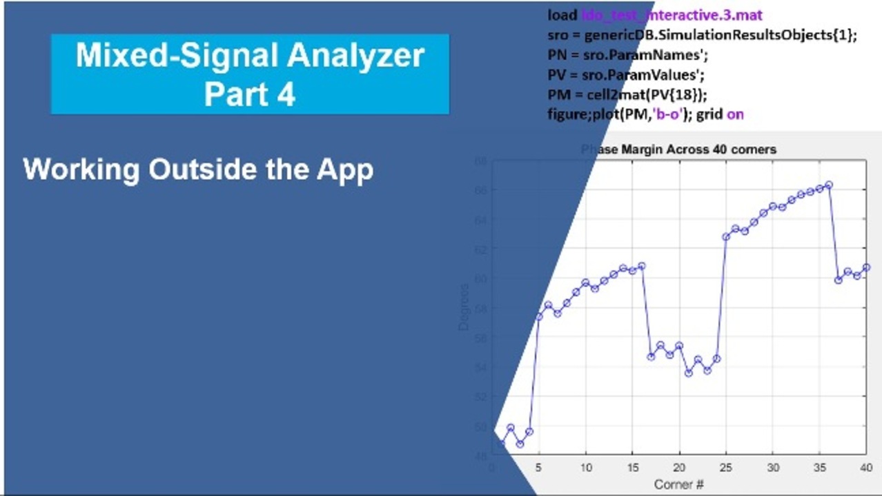
In this case, it's 40 cases. So, that's why you see a 1 by 40 cell. All right, and then, after that, we see some of the metrics that we computed. So, phase margin is element 18. This would be 12, 13, 14, 15, 16, 17, 18, is phase margin. And that's where the phase margins were computed for each case, for each variation in current capacitance, process corner, temperature, and voltage.

And this is just a short script in MATLAB, which pulls out that data I'm pulling out. The phase margin data, I convert the cell array to a MAT vector. And then, I plot that out, OK? And so, that's all I'm doing there. We're going to jump over in MATLAB and see that in a second. And I'll just show you the phase margin trend chart that we did in Mixed-Signal Analyzer. We did that in a previous video.

And then, I'm showing the equivalent thing when I run that script that I just showed you on the previous slide. I just recopied it over here. The tricky part of this, or the tedious part of it, is decoding the order of those variables. So, for instance, current load, capacitance value, process corner, voltage and temperature, in order to make one of this plot over here, where I just plotted parameter value, which is phase margin straight, versus the way I customize these categorical x arrays over here in Mixed-Signal Analyzer, the tedious part is to get these to match up with the straight plot of the data.

So, you have to know how the data is stored. And we don't really, again, have documentation on that. It's kind of a pseudo, kind of a manual process to look at the plot in Mixed-Signal Analyzer and look at the plot coming out of your MATLAB script and saying, OK, now, I know the order based on these x-array orderings over here.

All right, so, let me go on over into MATLAB. And we'll look at this a little bit more. All right, so, let's take some of the data. Let's just load ldo_test_ complete. I'll pick three. As before, you'll see the waveform data pointer, not the data itself, but the pointer to it, and then the metrics data. So, I will do what I did before. I'll say, sro is equal to-- and I'll just grab, GenericDB simulation results objects of 1.

When I do that, you're going to see many fields here. The one I'm most interested in, again, is that simulation. If I just type GenericDB, maybe I should just do that, to show you that. The one I'm most interested in is the simulation results objects. So, I pull that one out. I wasn't necessarily looking at the others right now. So, I have sro now. And the ones I'm most interested in are ParamNames and ParamValues. And that's what I had in my script earlier.

I just pulled those out. And I could just say-- and I'll do phase margin as well while I'm at it, evaluate those. So, now, ParamNames, ParamValues, and phase margin data. And the phase margin data, I've already converted it to a MATLAB vector. So, those are our phase margin values for this particular test. All right, I think that's all I'm going to cover in this video.

And I hope it's helpful. And just keep in mind that the accessing of raw data is still an undocumented feature. So, you won't be able to look into the doc and find it as of R-2023b. But in the future, I think we'll have some easier ways to access it. All right, thank you very much for tuning in-- signing off.