RF Data Analysis and System Design for Scientific Applications, Part 2: Design and Budget Analysis of RF Systems

Next month, we're going to dive into chain analysis, including nonlinear components. So, so far, we only talked about S-parameters and linear behavior distributed or lumped. What about nonlinear components, such as amplifiers, mixers, or different types of behavior? So, so far, we talked about passive components.

And, by the way, had a question about the switches. And switches are-- you could consider them as linear, but they are time variant. So a component that is a linear time invariant can always be analyzed, essentially, with a transfer function with S-parameters. Everything is easy. As soon a component changes its behavior in the time domain or a component is nonlinear, effectively, it a time-variant linear component essentially becomes like a nonlinear component. So we need to do something different.

So where do we start, in this case, if we have components that are nonlinear or components that are time variant? Do we start with the RF Budget Analyzer App or RF budget analysis? I think that in my experience over the past 10 years, every single RF design that I've dealt with always start with some sort of budget analysis, often done with spreadsheets. You have the different components, gain, maybe nonlinearity, maybe noise figure. You put the chain together and then you analyze it.

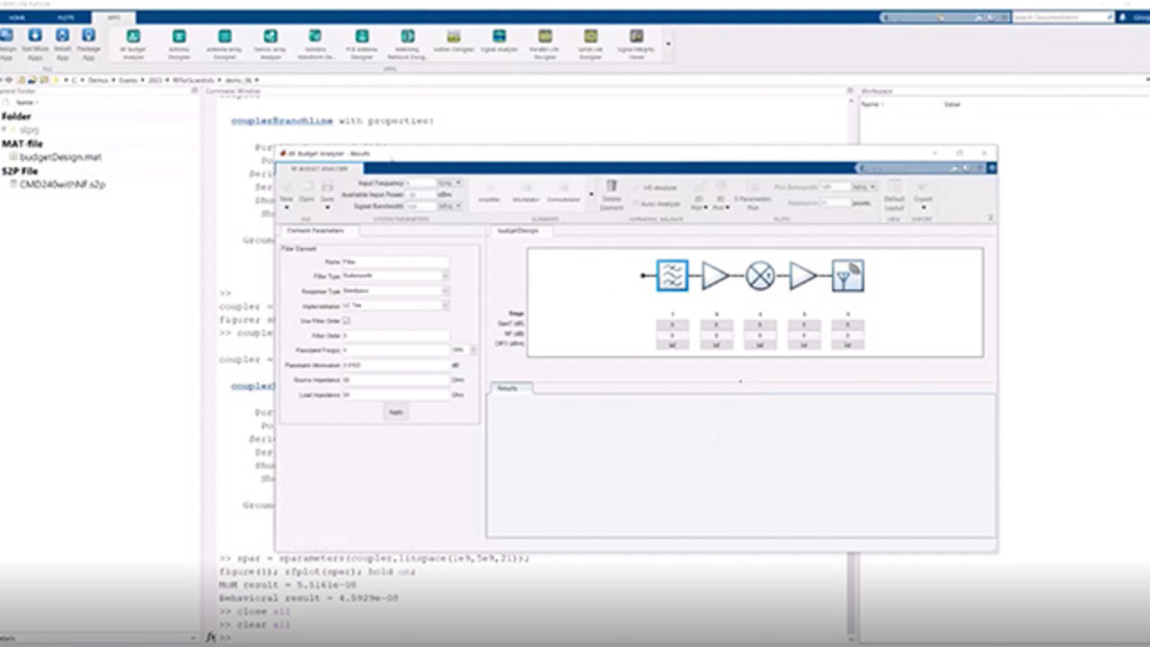
With MATLAB, we provide the RF Budget Analyzer App where you can essentially look at the lineup of the different components. So, for example, here, you see in this figure, we have five different components. For each of the components, we have what is the gain, the noise figure of the IP3. And then we look at the budget of the component 1, component 2, component 3, component 4, and see how this propagates through the chain.

I would say that the Budget Analyzer App that you find in RF Toolbox is a little bit better than what you normally do in Excel because it also takes into account impedance mismatches. So if you have S-parameters-- like, in this case, for the filter or for an amplifier-- then the impedance mismatch has an impact on the power transmission as well as the noise transmission.

Again, it's an app, is graphic, but like all apps in MATLAB, allows you to generate a script. Again, another finding that I want to share with you is that in my experience, point and click is always great, but everything that can be automated is even better. Because it's more traceable, it's easier to understand, it's easier to reproduce, and it's easier to share. And what this app also provides-- and links back to the question to it allows you to generate a model that can be used for time domain simulation and system integration.

So instead of using PowerPoint, now I'm going to go back to MATLAB. Just stay with me. I'm going to close all figure, clear all variables, close my demo, and then go to one new demo. And what I'm going to do here, I'm going to a start up or fire up the RF Budget Analyzer App-- probably is the most used app, at least, for me.

I always start here. And during the evolution of a design, I tend to go back to the budget analysis a lot. What does it mean? You start with a budget analysis and then throughout your development process, you tend to evolve the model, the simulation model, maybe because you have more information, maybe because you have measurements. So sometimes you start really top down with your specifications, then you get measurement, and then you start absorbing the measurements into your model.

But it's always important that whenever you evolve the model, you need to land on your feet. You need to check that the results make sense. There are lots of things that can go wrong. Sometimes it's just-- most of the times, I would say, is human mistake, like you look at the wrong frequencies, or there is an undesired impedance mismatch effect. Or maybe you have an antenna array and you're looking in the wrong direction. You're not looking at both sides.

And then all these type of things have an impact. And they need to be validated and verified against the budget. OK. So let me open up a budget that I computed before, simply because it makes it a little bit faster. What do we have here? Budget analysis is, by definition, the analysis of a single chain. We look at single input, single output, and we see how the chain propagates.

So in this case, you see we have-- OK, let's start from the top. This is a good place for it to start. So I know that the input frequency is centered around 4 gigahertz with available input power in this case, or minus 30 dBm over a signal bandwidth 100. These are just the system specification that tells you what is the characteristics of my input signal.

Then we have a bunch of components here. I have five components. I could have added amplifiers, modulators, filters, parameters, transmission lines, antennas, RLC networks, attenuators. In this case, the first component is a filter. It's just a Butterworth filter band path of order 3 between 3.5 and 4.5 gigahertz, followed by an amplifier.

For the amplifier, I provided the gain and the noise figure. And the output refer the IP3, that is a measure of nonlinearity. If you had S-parameters-- you can also, for example, specify S-parameters for your amplifier. Just to give you an example, that would take into account impedance mismatches at the input and at the output, as well as frequency dependency of the gain and also reverse isolation. In other words, the fact that is a single chain, it doesn't mean that is-- essentially, if there is an impedance mismatch, part of the energy will be reflected back through your chain.

Let's go back to where we were. Oh, I forgot this one. I forgot 15 gain, 2.9 and 28. That is where we were. OK.

And then we have a modulator. The modulator, in this case, again, you can treat it in a first instance as an amplifier in the sense that it has a certain gain, a certain noise figure, and certain output IP3. But it also does an up conversion of your input signal with around a local oscillator frequency of 23 gigahertz, which means that the output of the modulator, we enter at 4, we add 23, we end up at 27 gigahertz-- followed by a power amplifier again but specified by its nonlinear characteristics.

We can also plot the characteristics just to give you an idea on how the power amplifier behaves and then terminated onto an antenna. So you will see that this power amplifier, for example, will saturate around 37 dBm of output power. And then we have an antenna that we can-- I'm not going to talk about antenna design simply because I want to keep it a little bit short in terms of presentation.

But for you to know that everything that we have seen for the PCB components, we have a similar approach for antenna design. So we have a catalog of antennas that can be analyzed using the method of moments. In this case, I designed a circular antenna and used the results of the electromagnetic simulation integrated directly into the budget.

Very good. So let's look at the results of the budget for a second. What do we have here? We have the output frequency. So you see that if you have components such as modulator, on the modulator, the output frequency will change. By the way, if you do have direct conversion architectures, so architectures that convert to I and Q or that starts with I and Q, this is also supported. That convert around that 0 Hertz or DC.

And you see here at the budget here at the bottom how, for example, the gain-- so after the first filter, the filter essentially has a gain of 0. So the gain of the chain is 0. The amplifier's, again, at 15. So this is fairly straightforward. You see how the gain of the chain is essentially the sum of the gains of each of the components.

Similar, the noise figures used is determined using Friis equation. So the noise figure of the first element has more impact than the noise figure of the next element in the chain. Because every element noise figure gets divided by the gain of the previous elements in the chain, as well as IP3 and the overall signal-to-noise ratio.

We can inspect our network, for example, by looking at the S-parameters. This also can be interesting. We can see how the S-parameters propagate through the chain. So one of the things that, for example, I find very useful here is to see if the response of the system is flat in the bandwidth of interest.

So, for example, here, I'm going to increase the bandwidth to 800 megahertz so I can inspect here if my response is flat in the bandwidth of interest or if there are reports. If there are reports, then this might cause distortion to your signal that you might need to equalize, for example. Or you might need to compensate for a group delay, just to make an example. You can look at the S11, S22, and so forth on plots, equivalently, as well as you can look at the reverse isolation as well.

One last thing that I want to mention that is very important and is something that goes beyond what you normally do with spreadsheet is that we can analyze the chain using harmonic balance. So what is harmonic balance? Why is it important? Harmonic balance is a nonlinear analysis.

So, so far, we looked at the chain, and we computed the results of the chain using Friis equations. So Friis equation, I would say, is what we all learn-- at least, in engineering schools. It's a very simple way to look at the budget in terms of power, noise figures, and IP3. And they are simple, basic formula. I would say these are the formulas that every single engineer implements with a spreadsheet.

They are theoretical formulas. And for the gain, it's very straightforward. The output the gain is just--

[AUDIO OUT]

--type of representation. However, this type of representation essentially has a number of assumptions, first of all, doesn't explicitly model the impedance mismatches. So if you want to model impedance mismatches, you have to measure the gains, taking into account the impedance mismatches.

Doesn't say anything if I have up conversion or down conversion. And I can tell you that doing a Friis analysis of a conversion, the conversion can be tricky because, for example, it depends on, do I have image rejection filters? They're important because then they will take into account the impact of, for example, noise in the image bandwidth, yes or no. There can be a difference of 3 dB, twice as much noise. And suddenly, you don't know where it's coming from.

But also, these equations assume that each of the elements are operating in linear or quasilinear condition. So if we are close to saturation, these equations don't hold anymore. So let me just go back to my budget analysis. So I computed the harmonic balance results.

And you can see here in this case that I'm comparing next to each other, one to each other, the results of Friis and harmonic balance, power gain in this figure. And you can see the numbers are actually very, very similar. Why is that? Well, because the input power is relatively small.

So, if you remember, when we look at the power characteristics, for example, of this amplifier, we saw that this amplifier saturates around 37 dBm of output power. Now if I look at the output power at the end of the four stage, we are 16. 16 is well below 37, which means that we are operating, essentially, in a very linear condition for this amplifier. So we are very far away from saturation.

And in this condition, yes, results of Friis and harmonic balance are in good agreement. This is exactly a confirmation that we are operating in the region-- on the operating region of our network that we are expecting. So we can try something a little bit more exciting. If I increase now the input power from minus 30 to 0 dBm-- now I'm increasing by a factor by 30 dBm, which is a lot-- if I now repeat the harmonic balance analysis, I would be much closer-- or actually, above that saturation level, and then Friis results will not hold anymore.

So what is harmonic balance? Harmonic balance is really known linear analysis, is the foundation, essentially, for every nonlinear simulation that you perform in RF systems. Essentially, it consists of a steady state [AUDIO OUT] applying sinusoidal tones at the input and looking how this essentially-- how the nonlinearity in your system affects these sinusoidal tones.

And it allows you, essentially, to predict the effects of nonlinearity, of saturation in the modulation effects as well. So, for example, if you have a mixer with different mixing terms, you will see the results with harmonic balance. We provided an RF Budget Analyzer. And this is also the foundation that is required for circuit envelope simulation. That is the technique that I was talking before that we can use for time domain simulation of nonlinear components, including switches or time-variant components.

Now if we go back to RF Budget Analyzer App, I can now compare the results again. And you can see that now, for example, the output power with the harmonic balance is much below what Friis was predicting. So Friis was predicting 45. We are actually getting 36. And that's right. Because essentially, our power amplifier here was actually clipping at 36.

We are now operating in saturation region with an input power of 30 dBm, so we are somewhere here up in the region, which means, essentially, that Friis conditions are not satisfied anymore. Why I'm showing this? Because, again, you always need to check, you always need to verify the results. A simulation model is very important. It's very helpful to predict how your system is going to behave. But you need to gain trust that the simulation model makes sense.

In many cases, I worked with users that put together a simulation model and then they start streaming a very complicated waveform. It could be a new FTM waveform. It could be a standard compliant communications radar system or a pulse waveform. And then they're looking at the results, and they don't make sense because they're very different from what their Excel spreadsheet is telling them.

So is it an error of the simulation? Is an error of the simulator? Well, it's not an error. It's how the system behaves. Nonlinear effects do have an impact on the behavior.

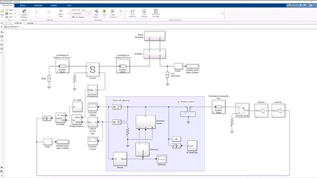
One last thing that I want to show you from this app is that not only it allows you to analyze a system, but it also allows you to generate a model. And once we have this model, we can now do very interesting things. We can start putting this model into a larger system. We can close it in feedback loop. So we can start looking at complicated scenarios, if you like, just like our inner particle accelerator that we saw before.

So in this case, what we have here? We have the chain of the components that we had in RF Budget App. So you see they have the same five components. We have a very simple testbench. But, more importantly, we can now execute this model in the time domain using an RF simulation.

So let's talk a little bit about this. So we generated our model. What is circuit envelope? Circuit envelope is a technique that is used to simulate RF systems. Now, when we talk about RF systems, RF means Radio Frequency. It means high-frequency signals.

Now, we are all familiar with Nyquist. So if you have a signal, you need at least two megasamples per period, essentially, to describe the signal accurately. In reality, you need a lot more to have an accurate--

[AUDIO OUT]

--the time step, realistically, that is 1 divided by 80 gigahertz, which is very, very small.

Because you need some oversampling, just like we saw before with rational fitting. Circuit envelope, which would mean, essentially, I need a timestamp that is commensurate to capture this orange waveform that you see here in the slide. A circuit envelope allows you to, in a way, ignore what is the center frequency or what is the carrier frequency of your signal and analyze that with harmonic balance. That is the technique that we saw before.

And it allows you to describe or to use the timestamp that is proportional to the envelope of the signal or to the modulation of your signal. And in general, those modulations occur at a much, much slower rate than your actual center frequency. So, for example, if you have a switch that changes the behavior not at the rate of the sinusoidal but at the rate of the envelope, you don't want to describe the switch with a lot of timestamps. That's the bottom line.

A good way to see the circuit envelope is a trade-off between an equivalent baseband representation-- that is, an IQ representation of your signal-- and a true pass-band or a real pass-band simulation where you simulate everything from 0 to the highest frequency in your simulation. Circuit envelope is in between in terms of abstraction. It's more general than equivalent baseband because you can have multiple carrier frequency. You can have multiple mixing effects.

But it is, of course, less faithful in terms of fidelity than real pass-band or true pass-band because it only captures, essentially, your signal of interest. So if your spectrum is sparse, circuit envelope is a good trade-off. Again, it's a trade-off. Like always say, there is no free lunch. Everything comes with a trade-off. But you, as a user, as a modeler, need to be in control of the trade-off to be good enough for your assumption.

How does it work? Well, essentially, you can specify as many carrier frequencies as you want. Harmonic balance will operate on the carrier frequencies. So like we were saying before, static analysis of CW tones, the carrier frequencies are analyzed with harmonic balance. The envelope or the time domain volume modulation are simulated in the time domain with a transient simulation.

In this way, you can look at all the mixing products. You can look at all the effects of nonlinearity, but the simulation speed will be faster than just looking or using a very, very small simulation time step.

Good, so--

[AUDIO OUT]

--create a model from the Budget Analyzer App. By the way, such a model, you can also construct it by just putting together your components. That's absolutely possible.

You can start with a blank canvas, and Simulink can connect the components. I find it easier to generate it from the app because then I have a setup that, to start with, is ready, is set up. But you can see here that from RF Blockset Circuit Envelope Library, we have all the components. We can just drag and drop the components on our canvas and create our own model.

The next part of the presentation is talk more about this, so using circuit envelope for integrating RF control components or RF components with control algorithms at the system level.