RF Design of Wideband mmWave Beamforming Systems - MATLAB & Simulink
Video Player is loading.
Current Time 0:00
Duration 46:27
Loaded: 0.36%
Stream Type LIVE
Remaining Time 46:27
 
1x
  • descriptions off, selected
  • en (Main), selected
    Video length is 46:27

    RF Design of Wideband mmWave Beamforming Systems

    Overview

    The current trend for wireless systems to operate at millimeter wave (mmWave) frequencies and over wide bandwidth drives challenging requirements for RF front ends. ​ In this webinar, you will learn how MATLAB and Simulink can be used for modeling RF and mmWave transceivers, performing RF budget analysis, and simulating wideband adaptive architectures. These will include RF components such as amplifiers, matching networks, and antenna arrays operating at mmWave frequencies.

    Using virtual prototypes, we will simulate wideband transmitter and receiver behavior including co-existence and interference scenarios along with beam-squinting and antenna coupling. These same virtual prototypes will be used to perform dynamic EVM measurements for different communications standards such as 5G FR2.

    With practical examples, we will demonstrate how to optimize baseband signal processing algorithms and control logic together with RF transceivers to compensate for RF impairments, to compensate for RF impairments, improve overall receiver sensitivity in the presence of interfering signals, and to support multiple communication standards.

    Highlights

    Topics that will be covered include the following:

    • Introducing MIMO RF front-end design including antenna arrays
    • Integrating antennas and PCB components into RF front ends
    • Modeling wideband mmWave beamforming RF transmitters and receivers
    • Simulating co-existence and interference scenarios

    About the Presenter

    Giorgia Zucchelli is the product manager for RF and mixed-signal at MathWorks. Before moving to this role in 2013, she was an application engineer focusing on signal processing and communications systems and specializing in analog simulation. Before joining MathWorks in 2009, Giorgia worked at NXP Semiconductors on mixed-signal verification methodologies and at Philips Research developing system-level models for innovative communications systems. Giorgia has a master’s degree in electrical engineering and a doctorate in electronics for telecommunications from the University of Bologna.

    Recorded: 16 May 2023

    Hello. Today, we're going to talk about the RF Design of Wideband Millimeter-Wave Beamforming systems. My name is Giorgia Zucchelli, and I'm a Product Manager at MathWorks for their mixed signal area. I've been in this role for more than 10 years. So there is a good chance that we already talked in the past, or we might have met in person at conferences such as the European Microwave Week or IMS.

    So why are we talking about millimeter wave systems? Why is millimeter waves even a thing today? Well, communication systems are driven to provide higher and higher data rates, and one way to do that is to use signals with larger bandwidth, and one way to support larger bandwidth is to move the center frequencies to higher frequencies in the millimeter wave range, the double-digit gigahertz range. We see this with far FR2 bandwidth provided by 5G and even more extreme trend for 6G.

    We see this in satellite communication systems where there is an explosion and using complex modulations such as DVB-S2X or 5G for nonterrestrial application, and we also see this for wireless localization systems that also require wider bandwidth for improving accuracy for providing location.

    The design of a millimeter wave system is complex. So first of all, propagation losses are higher, which means that you need to pack more and more antennae close together in order to develop beamforming algorithms that compensate for coupling effects. The behavioral system is not flat across the signal bandwidth with signals that have bandwidth exceeding 100 megahertz, easily 400 megahertz, 1 gigahertz, and more.

    So you need to develop equalization fixed-compensation linear resolution algorithms, and in the that's the system using CW or single tone, and this is not representative of the behavior of this system when it uses large signal bandwidth. This means that you need other metrics such as EVM, ACLR, and you need to measure this matrix in presence, for example, of different scenarios, such as interfering signals for receiver or when your system is really large with thousands of antennas, and this adds complexity to complexity.

    As a millimeter wave system designer, you need to answer many questions how many internal elements do you need? What type? What spacing? Is coupling affecting the system performance? How to test and design beamforming algorithm. What is the impact of dispersion? How to design and test equalization algorithms? What happens if a component fail, or if it's not compliant to the specification? What about interfering signals, and how do you scale up?

    In this presentation, we will answer all these questions and we will see how model-based design can help answer that. We will start with the design of a single chain this is our baseline. This is where we will start from and the array design then we will integrate them together into a larger system, for example, with 8 antennas and 8 chains, and then from there we will scale up to 1,000 antennas-- actually 1,024.

    So if you want to see how to simulate a full RF system with 1,024 antennas, stay with me. So we're going to see step by step the entire process starting from a single chain and increasing progressively the complexity of our model. We will use models throughout our entire design cycle. So let's get started, and this is going to be our first step.

    So every single RF design that I know of starts with, essentially, a budget analysis that normally is done with spreadsheets. In this case, we use it as a transmitter, as an example, made of five components, a filter, an amplifier, a modulator, a power amplifier, and finally, the antenna. It's a fairly straightforward system, but it's representative of many architectures.

    For each of the components, we provided specifications, like its s-parameters as well as linear characteristics in terms of output preferred IP3, noise figure, phase noise, as well as the impedance. So how do you do this in MATLAB, we use the RF Budget Analyzer app. There are many videos on The MathWorks website that show. In this case, we use a session that I previously created just to speed up the process.

    Here, you see the five components that we described before. It excited the input frequency of 4 gigahertz with an input power of minus 30 dBm and a signal bandwidth of 100 megahertz. For the amplifier. We actually use the s-parameters as well as the output referred IP3. At 4 gigahertz we see here the nonlinear characteristics. This is a component coming from Qorvo. It's just an example.

    For the modulator we set the low-center frequency at 23 gigahertz, so we do an upconversion from 4 gigahertz plus 23 gigahertz. We land at 27 gigahertz. Here, you see the budget at every step of the chain. So you see how each of the components modifies the budget in terms of power, gain, noise figure, and output.

    The last component of our chain is the antenna. We designed is the antenna using the Antenna Toolbox, so in this case, again, I load a design that I already did of a circular patch antenna. This is an interesting antenna for many points of view. It's just in free space for simplicity, but I could have mounted it on a dielectric.

    Here on the left, you see the geometric characteristics of the antenna. We can compute its impedance using the method of moments full-wave electromagnetic analysis. The s-parameters that give an indication of the bandwidth, as well as the 3D far-field radiation pattern. We see that the antenna is on the x-axis it has an activity of 9.7 dBi, pointing a 90 degree of azimuth along the bar side, and then we can update our element in the budget, and it gets updated, including the activity of the antenna as well as the final EIRP.

    We can analyze the chain using harmonic balance and s-parameters. We can plot the s-parameters across each of the stages of our chain, as well as we can use, say, the harmonic balance to look at the nonlinear characteristics of the chain. We're now going to export our budget to a simulation model. This is a Simulink model that we can simulate in the time domain. For each of the components, you can see that we have exactly the same parameters that we specified in the budget and the chain gets automatically created.

    The simulation uses a harmonic balance and circuit envelope in the background to compute the results. When we run the simulation, we also see that the output of the antenna is reported in both the vertical and horizontal polarization components, and we can now compare it with our budget and see that, with the simulation, we land exactly at the same place where we are expected.

    Now, we move from a single antenna to an array, and we will do a lot of studies of what coupling means with-- in the context of antenna design. So we go from 1 to 8 circular patch antennas. So we go back to our patch antenna that we just assigned to the session in the Antenna Designer app. We can verify that pattern. We can also look at the azimuthal part of the pattern with the antenna matrix. This is exactly what we just used in our budget. You can also verify the impedance.

    We are now going to export the pattern, but rather than exporting it as a measurement, we are going to export it as a script. This allows you to repeat the antenna design and analysis many, many times. Most MATLAB apps allow you to generate a script. We are going to modify the script to save the pattern of the antenna and the variable p. p is a MATLAB workspace variable that contains the magnitude of the far-field pattern of our antenna. It's a matrix of 37 by 73 elements representing the pattern of the circular patch at 5 degrees of resolution in angle.

    We are now going to open the Sensor Array Analyzer. From here, we are going to import our pattern. This could have been created with the Antenna Toolbox or it could have been generated by other third party electromagnetic software. We import our pattern that has been defined at-- with a resolution of 5 degrees. We use the variable p that we just created, and for the phase, we just use 0s in this case.

    The antenna was designed at 27 gigahertz that is the output frequency of our transmitter and this will determine the spacing in between the antenna elements. After we import the antenna we start with the design of the array. So we design an eight-element array spaced by half-lambda. We align the elements along the x direction, as we have seen so that our array normal is along the y direction of-- or 90 degrees along the azimuthal direction.

    Once the array is designed we can compute the far field the radiation pattern using pattern superposition of the isolated element. It's a little bit jigsaw because of the resolution of 5 degrees. We can inspect the pattern. We can also look at the azimuthal cut to verify that is pointing at 90 degrees. From here, we measure the directivity and 90 degrees along the azimuthal direction, and we see that we went from 9.7 to 16.3 dBi using 8 elements.

    Let's say that we are happy with that. What's next? We are now going to verify two things. First of all, what is half lambda? In this case, half lambda is the light speed divided by the operating frequency divided by 2, so 5.6 millimeters. Now, we are going to use the Antenna Array Designer, and we are going to verify that this spacing is possible, and we're going to verify that the pattern what we saw with the Sensor Array Analyzer computed with pattern superposition is actually accurate and representative of the full-wave analysis of the antenna.

    I open the Antenna Array Designer, and first of all, I see that I have my eight circular patches and that I cannot have a spacing of 5.6 millimeters because the antennas would touch, so I need a larger spacing of 6.4 millimeters. So I cannot verify my far-field pattern, and I can see that the directivity is 16.3 dBi, close enough to what we just obtained with the Sensor Array Analyzer, but the pattern, it looks at looks very similar on the main lobe, but on the side lobes, it's slightly different. This is due to the effects of coupling between the antenna elements.

    We also computed the parameters of the array, as we have 8 elements. We have 8 by 8 64 as parameters representing the impedance, the bandwidth of each of the antenna elements, as well as the coupling. So now, we will use this information to verify that our antenna array analyzed with pattern superposition provides consistent results, and also, we will use the parameters to model the near-field coupling of the antenna element.

    So we go back to our Sensor Array Analyzer session, and we change the spacing in between the antenna elements from half lambda to 6.4 millimeters. We see that the directivity is slightly different, but more importantly, because now we are at more than half lambda, we will have grating lobes, and remember, grating lobes cannot be minimized with tapering. So far, we saw the effects of coupling or going from one antenna to eight antennas. Now, we're going to see the overall system performance by integrating this 8 and 10-element design with our transmitters.

    So this is the same design that we just generated from the Budget app. We remember the ERP of 25 dBm along the horizontal position. I created a model, for convenience, where I copied this chain eight times. This chain is independent, so there is no coupling. We just sum up the power at the output, and what we see is that we land at the output power of approximately 43 dBm.

    This is the EIRP that you would obtain if you would do a simple static analysis using spreadsheets. Now, we modify the design to use the s-parameters of our array that we just computed with full wave electromagnetic analysis. These parameters now compose the eight antennas and models the near-field coupling.

    For the pattern, we use pattern superposition. We use, again, our variable p, representing the pattern of our patch, eight elements spaced by 6.4 millimeter along the x direction, and we can verify, again, that this provides the same pattern that we just analyzed with the Sensor Array Analyzer. So we use pattern superposition of the isolated element to compute the array k and its activity. So we take into account the near-field coupling but not far-field coupling. We run the simulation and will end at the total EIRP that is approximately 40.3 dBm.

    In our last model, we use the antenna block. The antenna block allows you to model both the impedance of the antenna array as well as the near-- far-field coupling. So we use the object patch_8_array. This is our array of eight circular patch antennas the same array that we just designed with an Antenna Array Designer with Antenna Toolbox.

    The antenna block does all the work for us to take into account both near and far-field coupling and this really gives us the ultimate measure of what is the impact of coupling. We run the simulation, and we end up with an EIRP of 41.5 dBm. So you can compare now what is the effect of near-field coupling and compare it with no coupling at all, this gives you an understanding of where the coupling is coming from.

    Also, remember each antenna behaves differently. If you would have done this with dipoles, dipoles don't really couple so we wouldn't have seen such big difference, and 3 dB is half the power, so coupling is definitely something that you need to take into account in your system performance.

    Now, we're going to extend the models to include beamforming algorithms, and we are going to see the impact of nonidealities introduced by the RF transmitter on the beamforming algorithms. We go back to our Sensor Array Analyzer session. This is where we landed before with our array pointing at 90 degrees with a directivity of 16.9 dBi. We now steer the beam at 30 degrees from the Bohr side. This will allow us to compare the amplitude and phase excitation to steer the beam.

    From here, we are going to generate a script again, like we did before, and we will get something similar to this, where we use our an 8-element ULA with our custom antenna element with our pattern p, and we can compute the phase shifts. So the variable phase shifts now include the eight phase shifts that are required to steer the beam at 30 degrees from both sides, 3 minus 100, and so forth.

    Now, we go back to our model that we just created, and we are going to make-- modify the model to include the phase shifters, and each of the phase shifters use the phase shifts to steer the beam. Now, we're on the simulation and we end up with an EIRP of approximately 39 dBm 39.6.

    We also modified the model to sense the voltage excitation at the terminal of each antenna. So this output port probed the complex excitation at 27 gigahertz that each antenna receives, and we save it into the variable workspace called Vout.

    Why is this useful or interesting? Because now, we can use the variable Vout as an excitation in amplitude and phase to our antenna array. This is the antenna array that we analyzed using full-wave electromagnetic analysis. In other words, this allows us to look at how the pattern of the array looks like instantaneously, depending on your excitation.

    We can see the 2D as well as the 3D pattern as well as the antenna matrix. This is a very important step because now we can analyze the effect of the entire RF transceiver chain in terms of nonidealities on the pattern itself of our array.

    So let's see what I mean. We can, for example, change the output impedance of our amplifier. We can randomize it with a variable to be between 25 and 75 ohms. You can see here, we modify our model so that the output impedance of the amplifier is defined by a random variable, with the real part between 25 and 75 ohms and the imaginary part between minus 10 and plus 10 ohms.

    Now, we run the simulation multiple times. You see it here. We run it three times and three times we go three very different patterns. Similarly, we can change the input or the low-center frequencies. A low frequency in this case is 23 gigahertz. The input frequency is 4 gigahertz. These are variables that are defined in the workspace. We can change them. This means that our antenna array that was designed to operate at 27 gigahertz will be excited at 27.5 or 28 gigahertz, and this will lead to deformation to the pattern itself due to mostly dispersion.

    We could also change the input power of our chain and drive the transmitter into saturation. So here, you see how we saturated the device, the transmitter, so the output power is not what we would expect but is lower, and we can see the effect of nonidealities cities on our pattern. We can verify, again, at each step that the simulation and the budget analysis provide consistent results even in saturation.

    And by the way, if you looked at the budget, you could see how we are here comparing freeze results with the harmonic-balanced results and harmonic balances and nonlinear analysis. So we see the impact of saturation on the budget itself. Again, you see how at every step I went back to my budget and compared with simulations.

    So far we've had each individual chain separately. This is not realistic. In reality, we will have one input signal, and we will have a feeding network. In this case, we modify the design to have a Wilkinson splitter as a place order to the network, and we are going to measure here the EIRP that is approximately 38-- 39 dBm.

    The Wilkinson introduces as a flat behavior in frequency, so it's constant in frequency. It includes a phase rotation and alternation of 9 dB. Now, we're going to design a Wilkinson splitter on a PCB using their PCB Toolbox. So we design the Wilkinson splitter we change the spacing in between the two arms so that we can cascade multiple chains and create a network that splits the input signal to eight outputs.

    So this is our Wilkinson splitter that we just designed. We see with seven lines of MATLAB code, as well as, we can expect, its parameters. Because we changed arbitrarily the spacing between the arms, these parameters don't look great. As you can see there is a little bit of tapering, and it's not well matched, but for the time being, we go with what we obtained just for convenience.

    We've got to design a second Wilkinson splitter, and we can, again, inspect its s-parameters and then we are going to cascade the first Wilkinson splitter with two instances of the second Wilkinson splitter that we just divided. So you see, again, we use PCB cascade. Last, but not least, we are going to design a third stage of the Wilkinson splitter. Again, inspect its s-parameters. Never going to going to look a lot better in terms of bandwidth matching and losses, and then we're going to cascade the three structures to create an 8-port divider.

    We computed the parameters, and we are going to use them in our model. So we go back to our model,. We are going to remove our placeholder in place of an s-parameter block. In the s-parameter block, we are going to use the variable sw that we just computed using full-wave analysis and the RF PCB Toolbox.

    We're going to use into sw into the s-parameter block. This data could come from a file. It could come from measurements. It could come from third-party vendors. We are now going to reroute and reconnect these parameters to our network, and again, verify the simulation. At every step, we verify that the results are representative of the budget of our transmitter.

    So far, we sort of cheated. We used the simulation but just to look at CW tones. Now, we're going to use wideband-modulated signals to test our transmitter. We are going to start with a simple OFDM testbench, a simple baseband transmitter and receiver that generates a random integer. Use a 64 QAM modulation. Use an OFDM multiplex with 1,024 carriers, each with 120-kilohertz spacing for a total of 122 approximately megahertz of bandwidth.

    We are going to upsample this signal interpolated with a factor of 4, so to look at the effect of spectral regrowth caused by the transmitter, and we are going to stream it through a baseband receiver that is going to downconvert it, equalize the gain, and apply coarse frequency offset, demodulate it and the carrier synchronizer, and we are going to, of course, look at the constellation and measure the EVM.

    We modified our model to include a new FDA test bench, If you look under the mask of the test bench we have baseband signal generation. That is composed by the blocks that we just saw in the slides. It also includes a power meter to measure the power and the spectrum analyzer to look at the spectrum of the-- at the input of the baseband receiver after the transmitter. We apply some delay, decimation, AGC, coarse frequency offset-- phase offset calibration. We apply the demodulator. We'll talk about the equalizer in a second, and then we also have a carrier synchronizer and the constellation diagram.

    When we run the simulation, what we see is-- by the way, the input signal streams to the input of our transmitter. The output is probed from the horizontal polarization of output of our antenna array block. We run the simulation. We look at the spectrum as well as we look at the constellation. The spectrum is measured over a wider bandwidth because of the interpolation factor of 4. So we will see a 100 megahertz signal coming in, and we will see the spectrum being updated as well as the measure of the ACPR.

    On the right-hand side, we see the constellation diagram. It takes a while for the AGC and carrier synchronization to lock and to recover the baseband constellation. The constellation diagram gets updated one with 1/4 of the speed of the spectrum analyzer because the signal needs to get decimated by a factor of 4, and on the right-hand side, you see the EVM measurement of the spectrum.

    You see that the constellation gets more compact, and as the carrier synchronizer locks, it gets closer to our reference 64 QAM constellation. By the way, in the diagram, in the model, you also see the EIRP converging towards our 38 dBm of EIRP that we were measuring before, and now we get an EVM of 1.5%. If we run the simulation longer we will get a slightly better result due to the locking of the carrier synchronization.

    What did we need it in equalization? Because our transmitter is affected by dispersion. So in the Budget, when we looked at the s-parameters we could have looked at the phase of the S21, and we would have seen a constant group delay of 30 degrees phase rotation over the 100 megahertz of the signal.

    This means that at every carrier of the signal, a different phase shift is applied by the system and the carrier synchronizer cannot compensate with this. We need an equalizer. So without the equalizer, we would have not been able to recover our constellation. So in this case, the equalizer just applies a phase compensation that is fixed and allows us to obtain a much better constellation.

    Things are fairly straightforward with a system that has just a 100 megahertz bandwidth. We did the same experiment with a 400 gigahertz-- 400 megahertz bandwidth, and things get a lot more complicated. So there is no such thing as a simple baseband receiver when we are talking about signals with such large bandwidth and such large frequency of operation. In other words, things get complicated. For this reason, in the remaining part of the presentation, I used a different baseband signal generation mechanism and different baseband recovery. So what I used is 5G standard compliant signals and the receiver.

    Here, I'm modifying the model so that the input and the output are not connected to anything. We just have an input port and an output port, and we will use this input port and output port to exchange waveforms to and from MATLAB. The input for waveform gets upconverted to 4 gigahertz and streamed through our transmitter. The antenna array probes the output waveform at 27 gigahertz. So this model has the name TX_8patch. Remember this because it's important.

    In a matter of workspace, I have a variable that is called RF_TX. RF_TX is an RF system that wraps our Simulink model, TX_8patch, with a given input frequency, output frequency, and sample time of execution. Now, I can use the RF system, RF_TX, to simulate our transmitter as part of a MATLAB script or a MATLAB testbench.

    To generate this test bench, I'm going to start from the Wireless Waveform Generation. This is the fifth app that we see today I'm going to use and generate a new radio test model-- a test a signal using FR2 bandwidth, and test model 1.1, that is representative for testing receiver, 120 kilohertz of subcarrier spacing for a total bandwidth of 400 megahertz.

    I'm going to generate the waveform, look at the spectrum at the resource grid, and then I'm going to export the waveform actually as a MATLAB script. From here, I'm going to use a this script to generate a waveform and test our transmitter using the RF system that we just saw before, and actually, I'm going to use some of the functions that are shipping as examples, not only to generate a waveform. But also to measure the EVM of our transmitter. So let's see it in action.

    At first, the generated waveform is good practice to verify what is the spectrum of our waveform. We're going to measure, in this case, the ACLR using the Spectrum Analyzer because this is a reference waveform. The only contribution to the ACLR is due to the interpolation filter. We need to interpolate the waveform because we are testing a transmitter we want to see the effects of the spectral regrowth.

    We are going to measure the EVM using, again, a helper function here, and we are expecting an EVM of 0 we get something really, really small. So it's good we scale the input waveform the 5G standard compliant waveform, TM1.1 to have an input power of minus 21 dBm, and then we are going to stream it through our RF system, RF_TX. That is the wrapper around our Simulink model.

    Notice that the Simulink model gets executed with a sample time that is 1.9 gigahertz. What is it? It's essentially our 491 megahertz divided by an interpolation factor of 4 or multiplied times 4. As we execute our RF system, we see, in the background, our Simulink model gets executed, and as the simulation progresses, we see the EIRP being updated live.

    We run a waveform that is one millisecond long through our transmitter, loading here the results that we are already precomputed, just to save some time, and I'm going to measure the output power the peak-to-average power ratio. I'm going to look at the spectral. You see the tapering, here, introduced by the Wilkinson splitter that was far from being ideal.

    We measured the ACLR on our spectrum, we see potential effects of spectral regrowth, and we use standard compliant functions to measure the 3GPP EVM. So we can see that now the EVM went from 0 to 7.6% due to the effects of the nonideality transmitter, and keep in mind that this receiver already includes automatic gain control and an equalizer.

    So this is what we are seeing. Essentially, we are seeing a way to include your RF models into MATLAB Test Benches and how to use a standard-compliant sophisticated baseband transmitter and receivers. We have seen this on an RF transmitter, but actually, we've also done the same experiment using developing a model of an RF receiver. So you see here that the model is flipped we have an antenna and a down conversion chain combining the signals.

    Why is this interesting? Because now that we have a model of an RF receiver and a 5G test bench that we can use to start to measure EVM and ACLR. We can also test quite exotic scenarios. For example, we can take into account interfering signals.

    So here, we're going to see an example where we test our receiver with a 3GPP standard compliant signal coming in at 60 degrees of azimuth with an input power of minus 70 dBm, and then we are also going to test our receiver with another signal coming in an interfering signal with 100 megahertz bandwidth with the same power, minus 70 dBm but coming in at 19 gigahertz and at 40 degrees azimuth.

    I chose 90 degrees because it's the image frequency-- our low-center frequency is 23 gigahertz. Our output IF frequency is 4 gigahertz. So 33 minus 4 makes 19. That's the image, and we will have a finite image rejection filter, and we chose 40 degrees because, in a way, this is the worst case scenario.

    If we are steering the beam of our antenna at 60 degrees at 27 gigahertz, due to dispersion and beam squinting, the beam will be deformed at 19 gigahertz and will be pointing at toward 40 degrees, so this is an interesting experiment. Without interfering signal the reference EVM of this receiver is 3.6 dBm 3.6%. Now, we will see--

    --on the simulation, that the dBm degrades. So we'll use, again, the same test bench that we developed before, but we'll use a different test model, a 3.1 that is more representative for testing a receiver. Again, we hop through the script quite rapidly. We look at the spectrum of the input signal, at the ACPR peak-to-average power ratio as well as the EVM. This is all done on the reference input signal, so it's all going well.

    We scaled down the input power to minus 70 dBm, and then we stream it through our RF system, RF_RX. This is an RF system that points to our Simulink model RX_8patch_OoB. The input frequency now is 27 gigahertz. The output frequency is now 4 gigahertz

    OK, I made a mistake. Let's open up our RF system, and let's look at our Simulink model. The magic happened here in the antenna block. You see we have two centers frequencies for two input signals and two different angle of arrival, 60 and 40 degrees of azimuth. So the desired signal at 27 gigahertz get combined with the undesired signal at 19 gigahertz.

    We also have an image rejection filter, which has a really large bandwidth, 21 to 27 gigahertz. So we'll have finite rejection at 19 gigahertz, and I didn't talk about it, but we also have phase noise in our receiver, just like we had it in our transmitter. The second signal is an OFDM signal that gets-- interfere with our 5G signal.

    We run the simulation, and now we look at the output power that, again, we verified with the budget of the receiver. The ACPR is not really important for the receiver, but we look at it in any case because it's always interesting to look at what happens to the spectrum of the signal, and now we measure the standard compliant EVM using our 5G Toolbox, and as you can see, the EVM went from 3.6% to 4% due to the interfering signal, and we can see here, in the spectrum, how the 100 megahertz bandwidth interfering signals gets mixed right in the middle of our desired signal due to the final rejection of the image rejection filter.

    From here, we can scale up to 1,000 of antenna elements. This is really the juicy part of this presentation. How can we do that. To do that, we need to raise the abstraction level of our model and we do this by breaking the model into three first of all, we isolate where the coupling happens in our model the coupling happens at the input with our Wilkinson splitter and our coupling happens in the antenna array.

    Then, we provide a higher abstraction level model for the transmitter chain or each of the transmitter chains, and we will run each of the transmitter chains using parallel simulation. What do I mean with raising the structural level of our chain? We're going to use five blocks and pretty much with these five blocks, you can pretty much model almost any transmitter or any receiver.

    The first block models the input preferred noise figure of our entire transmitter and this data comes from the budget analysis that we performed right at the beginning of this presentation. The last block models the output referred IP3 of our chain of 44 dBm, and again, this number comes from the budget analysis that we performed right at the beginning of the simulation.

    We also have an s-parameter block that models the dispersion of the phase and frequency dependency across the entire chain by cascading all the components that have frequency dependence. We model the phase noise of our modulator, and we explicitly model the phase shifters with an additional input because each chain that will be run in parallel will have a different phase shift to enable this to

    Let's see these in action. So this is the budget that we did right at the beginning we're going to use the numbers in the last columns. At the output of the budget, we are going to use the 3 dB of noise figure and the 44 dBm of output-referred IP3. I created, here an equivalent baseband band model where we use the noise figure of input referred, the output IP3 of the entire chain. We have a placeholder to represent the gain of the antenna block, a phase shifter for steering the beam once we have multiple chains. We model the phase noise with the mixer, and we have an s-parameter block that represents-- uses a touchtone file that we just created to represent the dispersion of our path reverse filter as well as of our amplifier.

    I have here a separate script, where we cascaded the s-parameters of the dispersive components. So we have s-parameters of our filters. We have the parameters of our amplifier we cascade them we computed the s-parameters of the chain, and then we save them in this touchtone file. So we will take into account selectivity, as well as ripple as well as phase dependence in bandwidth of each of the bounded.

    We now run the simulation. We verify the output power or the power at each stages of the chain will look at the noise floor that is the same with our accurate model on the top and our idealized model on the bottom. We also verify the IP3. Now, we verified that we could create an idealized baseband model at a higher degree of-- a higher level of abstraction, and keep in mind that this model doesn't provide exactly the same results but provides results that are similar enough.

    Now, we look at the coupling. We're going to model the coupling at the input and the output, and this is an example in your chain, you might have to break it in multiple places depending on where that coupling actually happens. We're going to do this using coupling matrix, and we are going to create this coupling matrices by looking at the s-parameters of the elements where coupling occurs.

    In this case, we model the insertion loss introduced by the Wilkinson splitter, and we're going to use the impedance mismatch losses on the diagonal of our matrix. On the off-diagonal elements, we're going to use the as s-parameters of the diagonal to look at the isolation. We do this for the Wilkinson as well as for our antenna array. This is a simplified way to look at the effects of coupling as well as impedance mismatch losses.

    So we go back to our testbench here, where we test our transmitter. Again, we hop through the first steps of the test bench quite rapidly. Will we generate waveform as k, the input power, and here, we are going to create our first coupling matrix. So remember, sw is the s-parameters of our Wilkinson. We use the elements on the diagonal to look at mismatch losses and off the diagonal to look at insertion losses and coupling effect.

    We multiply our input waveform of 5G standard compliant input waveform times our coupling matrix. Now, we're going to prepare the simulation for parallel simulation. So for each parallel simulation for each chain. We are going to create two time series the first time series represents the input signal. The second time series represents the phase shifts to control the phase shifter so that we can steer the beam.

    And by the way, what are we going to use if we are going to simulate the model TX_1? That is our idealized baseband model that we just verified. We're going to use the parsim to run eight parallel simulations and at the output, we are going to look at the output. You see this is the output power of each of the eight chains. Each power is slightly different due to coupling. We're going to couple the outputs using the output coupling matrix that we just computed using the s-parameters of the antenna array, and then we are going to combine the signals using an 8-element ULA with the uses our patch antenna pattern.

    We measure the output spectrum. You see the tapering due to the parameters. You see the spectral regrowth we also measured standard-compliant EVM using the 5G function. So far, what did I do? Well, actually I repeated the same simulation that we did before because we have already done the simulation brute force by using the full simulation of the entire array, including the s-parameters of the Wilkinson splitter as well as the antenna array.

    In other words, I just validated that my behavioral model of the chain, as well as a representative model of the coupling matrix is good enough. I compare the results. They are closed. They are not exactly identical because the models are different. The model on the right, operates at a higher abstraction level but this is good enough and it allows me to extend to 1,024 antenna elements.

    So you can see here how I can quickly go from 8 elements now to 1,024. You can see here on the left how we modify our script around 1,024 and 10 elements, and if you have a good computer with lots, of course, the simulation will be batched faster. We use parsim to run the simulation, and actually, we use the infinite array patch approach to compute the pattern of the antenna-- of the embedded element inside our antenna array, and then we combine the results.

    To look at the output power, we-- of course, we always kept that same input power, so now the antenna array has a very, very high directivity. So actually, we are actually going to get a lot of power at the output, but we can now verify the spectrum as well as the EVM. This approach, of course, is very flexible, but it also requires you to have a good understanding of where the coupling occurs, where the dispersion occurs, and how to model it.

    So what can we say at the end of this long day. We have seen a lot, but what we are seeing is that at every single step, I verified using models, our simulation results. Designing millimeter wave systems is complex. Its physics there is nothing that we can do with that, but we can use models to verify that at every step, our abstraction level can be raised and can our model can be improved.

    So we understood coupling, dispersion, phase noise. We went beyond the textbook calculations, and beyond the CW matrix by using standard-compliant waveforms to measure EVM and the ACLR. We saw, for example, what happens when components deviates from the specification, and we gained insight into architectures and algorithms, for example, such as beamforming or equalization, before going to the lab, and of course, you can use such a model while you are in the lab to debug what is happening.

    With this, I thank you very much for your attention. I hope you enjoyed this long presentation and that you found it as entertaining as I did. Thank you.

    View more related videos