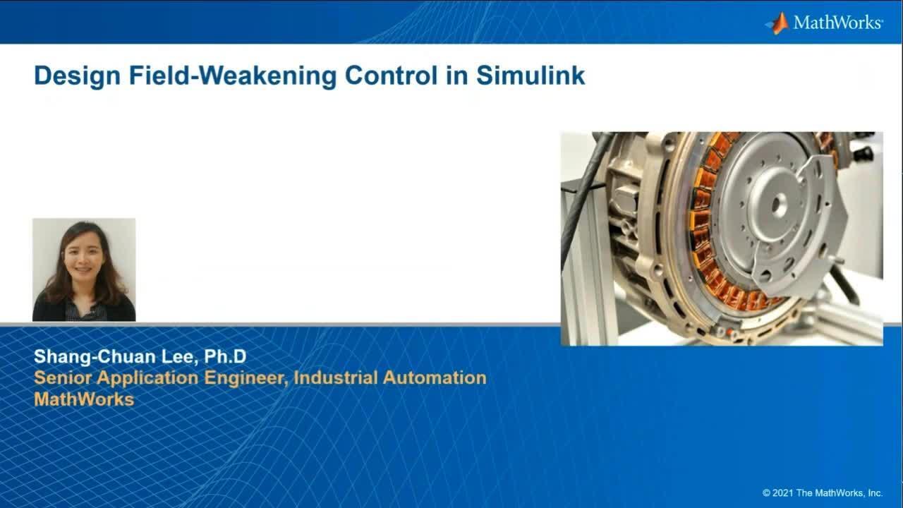
Simulate, Design, and Test Field-Weakening Control Design with Simulink
Overview
This webinar provides an overview of developing field-weakening motor control algorithms using Simulink. Field-weakening control is a technique for increasing the speed of an electric motor above its rating. Over-speed capabilities are required for motor applications in electric vehicles and locomotives and industrial automation when higher speed is required and lower torque is acceptable.
To simulate, design, and test field-weakening motor control on embedded hardware, this webinar will demonstrate two workflows. The first approach implements field-weakening control with a linear model and code-generation from the model for deployment on an TI C2000 microcontroller. This workflow uses Motor Control Blockset and is based on equations derived from a PMSM’s parameters. The second approach considers highly nonlinear nature of the machine where PMSM characterization tests are performed on actual hardware using a dyno setup or through an FEA tool. This workflow will show how to create a high-fidelity torque model with an automated workflow for calibrating the optimized lookup tables.
Highlights
In this webinar, MathWorks engineers will show you how to:
- Demonstrate two workflows for field weakening control
- Automatically generated code of the field-weakening control and spin a PMSM
- Calibration of the field-weakening control lookup table approach
- IPMSM field-weakening control explained on the id-iq plane
- Maximum-flux-based field-weakening algorithms
About the Presenter
Shang-Chuan Lee is a Senior Application Engineer specializing in Electrical system and Industrial Automation industries and has been with the MathWorks since 2019. Her focus at the MathWorks is on building models of electric motor and power conversion systems and then leveraging them for control design, hardware-in-the-loop testing and embedded code generation. Shang-Chuan holds a Ph.D from the University of Wisconsin-Madison(WEMPEC) specializing in motor controls, power electronics, and real-time simulation.
Recorded: 2 Nov 2021
My name is Shang-Chuan Lee. I will just get started with today's presentation. So before we get started, I would like to ask a question to everyone. Why do we need field-weakening control for electric motors, and what's the purpose of doing field-weakening control? Well the answer is, we are trying to achieve high-speed operations. From our literature review, they are many of proposed field-weakening control implementation on various types of machines, ranging from PMSM, permanent magnet synchronous motors, induction motors, to switched reluctance motor considering its cost and simple structure.
So what we see is that field-weakening control is not only popular in automotive industry for achieving high-speed constant power region. But also we see customers in industrial automation are also gaining inches of applying field-weakening control on their servo drives. But as you know motor control is a complex process, and there's so much more that you need to consider when it comes to design and implement field-weakening control.
For instance, when I was a motor control engineer working for variable frequency drive I need to perform various tasks ranging from plan modeling to motor control algorithm design. And I have to do multiple testing, verify on the real motor before our ultimate goal is to do mass production on the microprocessors. So our challenges we are trying to solve here is, can we accelerate motor control development process so that we can quickly spin a motor and validate our control design. So the answer is, yes. So this is what we are going to talk about today.
So in this presentation, I will introduce two workflows to design of field-weakening control. The first workflow I'm going to show you is how to implement field-weakening control in Simulink. And we will take PMSM as an example. So this workflow is an equation-based approach where control algorithm is calculated by lumped parameters. And this approach is suitable for those of you whom are interested in automatically generate C code from a model and spin a motor by an embedded processor.
So the second workflow is for high fidelity field-weakening controller considering non-linear effect of PMSM. Like I know some of you my in auto industry, we offer an automatic workflow for calibrating optimized lookup tables especially for a field-weakening torque control. And I will go through the workflow to show you how you to calibrate a control lookup table through flux data either from dyno testing or FEA modeling.
So let's just jump into the first approach. So like I mentioned earlier, motor control development process is really complex. It requires several steps before the final production stage. So the solution we propose here is an end to end motor control workflow to walk you through each motor control development stage with provided reference examples. And this is a great way to help anyone with a motor control background to get jump-started with their motor control project. But also these reference examples are also designed for generating optimized C code.
So as you can see, this work flow starts from current and position sensor calibration. It is I know some of you who might have experience designing motor control, it is a critical step before you design your closed loop current or speed controller. And then we will provide motor parameter estimation methods to help you identify unknown motor parameters. It is really helpful if you don't have motor data sheet.
And next we provide examples of a full-control algorithm design, such as classical field orientation control and also more advanced senseless control for different type of machine like induction motors or brushless DC. So until the end of this workflow, we also provide deployment and validation, which is the code production on the embedded processor. So here is the hardware setup that we are having for demonstrate this entire workflow, including a motor and inverter, how we are set up.
But what we are going to focus on for today's, is control design of a field-weakening control and deployment and validation side. For those of you who are interested in learning entire workflow and reference example we provide. They are supported by one of our toolbox, Motor Control Blockset. So you can find more information from this link. So before we jump into implementation of field-weakening control in Simulink, let's step back a little bit. How exactly we can achieve field-weakening control.
So the idea of field-weakening control is to achieve high-speed. So what I mean high-speed here is beyond base speed of the motor. As you can see from this torque-speed characteristic of PMSM, here on the horizontal axis is motor speed. And on the vertical axis, we can represent as torque, rotor flux, and stator voltage. So really the key here is base speed. So once our motor beyond the base speed, we are switching from constant torque region into field-weakening region.
Notice that before we reach to base speed, our stator voltage is proportional to the speed. And once we operate the motor beyond base speed over here, the stator voltage is constant, because we are reaching to inverter DC bus low voltage limit. So in order to keep pushing the motor to high-speed, what we have to do here is by reducing rotor flux, which can be illustrated on this diagram here by applying an opposite direction to the permanent magnet flux. So this is how motor can achieve high-speed constant power region. But in the meantime, we will sacrifice torque output as shown here.
So now let's see how we can exactly control Iq and Id current vectors in order to perform field-weakening control within its voltage and current limit. So based on the PMSM mathematical equation considering DC bus voltage and maximum current of inverter, we are able to plot this voltage limited ellipse and current limited circle. So our goal here is to produce maximum output power at maximum efficiency, so the current vector trajectories can be divided into three trajectories here.
So trajectory one is a long away curve, also called as, MTPA, maximum torque per ampere curve. What happened is when the motors speed is below base speed, so it is not required to apply field-weakening control. So by manipulating current vectors, trajectories along this curve, we are able to achieve maximum torque per ampere on this region. And trajectory two will be on this current limit circle from A to B. And trajectory three will be along this BC curve. It is also called as maximum torque per volt, MTPV.
This is when speed becomes very high by entering deep field-weakening. And the voltage becomes the only limit here. The current vectors go along the MTPV. So the area enclosed by 3 trajectory here, on OABC, this gray area is usually what we call field-weakening region. So regardless of the torque transient response you are given to your motor control system, your optimized field-weakening trajectories, or operating points will always be located within this gray area. And the key takeaway of this slide is to show you we can control multiple operating points on this current D2 plane.
So now let's take a look into more detail. How do we implement field-weakening control with MTPA? So as you can see from this controller block diagram highlighted in blue, this is an overview of closed-loop speed control based on field orientation control. But notice that in order to achieve field-weakening control with MTPA, we are going to focus on this particular block. And this block's implement is to calculate optimum current vectors along MTPA and field-weakening trajectories.
So with that being said, let me show you the control blocks we support from Motor Control Blockset library. So in particular, this is a blocks for generating reference current for MTPA and field-weakening. And these blocks support for both desktop simulation and Codegen for a fixed-point and floating-point data type. And we can further parameterize the blocks based on selection of either surface PMSM or interior PMSM.
So as we explore underneath of this MTPA controller reference block, in this case for surface PMSM, here you will see a schematic representation in Simulink blocks, is equal to mathematical equation for field-weakening control. And for achieving MTPA on the SPM motors, we know it's just simply command zero Id current. Before field-weakening control, the calculate Iq and Id currents need to be considered its inverter current limit.
And now what about implementation IPM machine? So first is for MTPA IPM. We can achieve maximum torque by computing Ip and Iq currents from a torque equation. So this is why maximum torque output includes a reluctant torque from return of Ld and Lq inductions. But as we keep increasing motor speed beyond the base speed, this is where our control algorithms switch to the model of field-weakening control.
And as you can see, these are the duration of mathematical equation behind for field-weakening control. But it just very high level the key point here is, we can calculate optimum Id and IQ currents based on voltage and current limits and maximum torque control algorithms. So if you are interested to learn in more detail of the mathematical equation that we use for this block, you can find the reference link from the slides, and we will share that with you.
So we just introduced the MTPA and field-weakening control blocks to derive Id and Iq current vectors. Let's see how we implement control algorithm in Simulink. So first you will see this is a speed controller and current controller of field orientation control. On top of that, we also have MTPA and field-weakening control blocks that we just introduced over here. But one thing to notice is that in order to have a stable operation for steady state and transient state operation, we also implement PI voltage regulation over here in order to identify the onset flux weakening.
So how it does is when the voltage vector is over the maximum voltage limit circle, the controller will sense the arrow of the voltage and it inject a d-axis current negatively to prevent the saturation of the current regulator. So this way, you can keep the current regulator from saturation by adjusting the flux level of the machine. So you can see that in our control algorithm, the Id current reference is made by the voltage limit control. And as for the current reference, it's also calculated within the current limit.
So now we have an accurate plan model and are ready to design our controller. So we will start with putting together field orientation control algorithm with MTPA and field-weakening capability. So let's take a look through our model. So the first things you will see is under the speed controller that compute Id and Iq current reference. So one thing to notice is that they field-weakening and MTPA controller block here, is it has input variables are calculate based on MTPA and field-weakening control. And the input variables are torque and speed, and the output signals are current Iq and Id.
And as we dive into the Id and Iq PI regulator, you will see this field-weakening controller is implemented by controlling Id reference. And it will feed a negative current to reduce the back emf voltage. Next I will navigate into a soft system that does sensory processing for current and position measurement. And these blocks are also supported by Motor Control Blockset.
Now I'm going to show you how do we compute duty cycles written to PWM driver blocks. Because this is meant for co-generation on the microprocessor. And here I would like to show you this is how we implement the physical plan model for the inverter and motor. So that we can run the full desktop closed loop simulation.
So after we design and implement field-weakening control and properly tune for PI gains in Simulink, here is the simulation result while we perform field-weakening control on the PMSM. So notice that on the y-axis, the speed and current feedback here per unit system. And as we increase motor speed of both one per unit at one second, the Id currents start to apply a negative current in order to achieve high speed operation. Right here starting at one per unit, one second, one per unit we are reaching to field-weakening region and the Id current start to applying a negative current over here.
So now let's take a look how we do experimental setup here. So the first thing is on the left hand side, we have this nice GUI interface from Motor Control Blockset. This allowed us to interact with the real motor control setup on the camera over here. And we have a power supply and inverter board, microcontroller, and a PMSM motor. So all the code, have already generated from a model, and it's already downloaded to a microprocessor.
So now what we are going to do here is we will just start pressing this start button and the motor will start spinning. And you are beginning to see how we are trying to slightly increase motor speed every 2000 RPM step. And now the base speed of this motor is around 6,200 RPM. And you will see the speed is increasing from this oscilloscope but also from the numbers over here. The current speed is around 10,000 RPM.
And as well, the oscilloscope is keep increasing the speed. And we are manipulating this constant blocks to increase the speed. So now the motors reaching to almost 18,000 RPM. It's like three times of the base speed. So we just stop the motors. Now you can see the motors are lowering the speed to 2000 RPM. So now after we stop the simulation, we can start doing post analysis of the system response.
So like here I'm showing you a speed loop response of comparing the reference speed and the speed feedback. But you can also log in to different type of signal, like phase current or torque, while you are performing real time control. So this workflow is showing you how you can quickly verify field-weakening control on the real PMSM motors. Because we are automatically generate a code from a simulation model and test immediately on the microprocessor.
So the demo I just show you is based on lumped parameter method, which means the model is rely on the set of mathematical equations and all the control design parameters are fixed. So this approach is suitable to initially verify your field-weakening control algorithm when you want to test some prototype motor drive system. I can give you an example from my customers in industrial drive application, they implement this method on their controller to test multiple motors to achieve high speed field-weakening operation.
However, if you are looking for high fidelity non-linear models like saturation effect, you will need to have another approach to achieve accurate torque control. So what do I mean by that? So well let's take an example here. So what impact of non-linearity and saturation does on field-weakening control operation. So let's plot field-weakening trajectory of traction IPM motors here.
So this is based on a linear motor model. And you can see the MTPA and MTPV operation and field-weakening region as I mentioned earlier. Imagine that we are designing an operating point of Id and Iq in the field-weakening region. And this operating point satisfies my initial torque requirement, as well as, both current constraints. Then I test on my IPM motor on the final setup and plot the actual trajectories here on the right hand side.
Now the exact same operating point, the same radars that are designed based on the linear model, falls outside of my actual dyno-tested field-weakening region. So the consequence is that first of all, you won't be able to achieve your torque accuracy. And most likely that operating point will violate voltage constraints. So you could end up losing control for your current. So conclusion here is that the optimal field-weakening point calculate from linear IPM parameters, may not be applicable to the actual motor due to the saturation.
So we cannot rely on linear model or linear lumped parameters to design your field-weakening control algorithm, particularly if you are doing high-power traction IPM. So what do you need to do is, you have to characterize your IPM on the dyno or FEN motor data. And then you need to calibrate your control lookup tables in order to achieve desired torque accuracy and efficiency.
So when it comes to calibration and field-weakening control lookup table algorithm, here is one of the popular solution which is maximum-flux-based torque control lookup tables. And it is using the control voltage and calculate for the maximum modulation voltage and compare with the DC bus voltage over here. And we will take the arrow through a PI controller where the output here is an adjustment of to a flux. And the flux here is used for adjustment of a regional maximum flux linkage, where it is calculated by maximum DC bus voltage.
And this algorithm is originally published in 2003 by GM. And by using this algorithm, clearly you can see flux levels adjusted based on the variation of the DC bus voltage automatically. Another key enabler of this algorithm are these two lookup tables. And they are maximum-flux-based Id and Iq tables. And the input of this lookup tables are torque reference and flux command for maximum flux linkage.
So how-- here is how we can implement this algorithm in Simulink. As you can see, we can use this to the lookup table as our flux-based lookup tables. And now the flux and torque will be the input and the output will be Id and Iq. But for today's, what I'm going to focus is not about control algorithm, because control algorithm itself is already well-established and implemented by many of industry.
So here instead, I'm going to show you a workflow. How do we calibrate these tables based on flux and torque? And because these tables are the key components of PMSM torque control algorithms. So now the question is how do you corroborate this torque control lookup tables? And the torque control lookup table need to be calibrated or optimized.
First I want you to know that there definitely is many multiple ways of doing this. I see customers using Excel. I also see customer using MATLAB script and even Python being used to calculate these tables. But I will place different methods into two groups. The first one I want to call in is full factorial and rule-based calibration method. And the second one is model-based calibration or MBC.
So what is full factorial and rule-based method? Based on our experience working with customers in auto industry in Detroit area and many start-up up company in Bay area. A lot of them are using this approach. So under this approach, we have to do-- The first thing we need to do is test your IPM on the dyno and varying the current vectors until you can achieve maximum torque.
And then they will need to repeat this many times for different magnitude of the current until you can trace this MTPA trajectory. But also depending on your field-weakening application, you might need to do more testing and operate on MTPV. And in that case, you need to test more datas in order to obtain MTPV trajectories as well. So with the defined envelopes and trajectories, you will have them graphically decide what is the best choice depending on torque requirements and speed level. And you need to integrate all this searching rules into your scripting.
Whenever the motor design is changed and you-- say if you have a new data set, then obviously the shape of this contours and operating envelopes may change, which will force you to adopt a new script to accommodate new design. So therefore doing this manually using rule-based and other code method require lots of dyno testing time and also in-depth domain knowledge in motor control, and definitely require lots of scripting.
So now that's why what if we have a workflow that can automate this process, not only increase productivity but also it is robust to different motor designs. So our proposed alternative is model-based calibration. So model-based calibration is an automated calibration approach that is already proven to achieve the same results with less time and effort. So first of all, let's talk about what is model-based calibration.
So it is the workflow for calibrating parameters for plant models and control systems. And model-based calibration includes the steps for the Design of Experiments, DoE, model fitting and optimization, design parameter tradeoff studies, and eventually, calibration generation for lookup tables. So when we use MBC, model-based calibration workflow, for these motor control applications, especially for PMSM field-weakening control, these are the steps we are going to use.
So we will start with DoE, Design of Experiment, and then data modeling. Then we can take advantage of the models and run optimization in order to achieve your predetermined objective, such as torque accuracy, maximum efficiency, and in the end of this workflow, we will implement this generated optimized torque lookup table to your Simulink whether you are using absolute torque speed point or percentage of the torque as the index to those tables.
So obviously we have this MBC toolbox can consolidate all these steps all together. So now I will just walk you through each steps in more details. And we will start with DoE. This is where you determine your testing point and perform characterization test on your dyno. So the MBC tools provide an interface for you to do DoE.
You can set up constraints for the DoE. So in this case, we set up the constraint for the currents. And the tools can create a pseudorandom operating point based on statistical sequence. And the most common one is Sobol sequence, which aims to strategically cover the designated space as homogeneously as possible and with this number of points.
And you can also augment the original DoE by selecting an area and generating more operating points. Like in this case, you know that around this area is kind of the tip of MTPA. And we know here is highly saturate, so we want to do more testing around this area. So what we can do is, we can generate an augmented DoE on top of original DoE.
So once you have a plan of DoE, and then you can execute it using either on the dyno testing or as an alternative, you can do if you don't have a dyno facility, then you can use FEA tools to execute your DoE plan. So when we finished the DoE, either on the dyno or FEA, we will lock the results into preferred format. And it can be an Excel spreadsheet, and then we will import them into the tool. And the tool will give you facilities to clean up and visualize test data. So in this case, what you see here is, we brought in the flux service and that's mapped on the Id and Iq plan.
So once we have all the data we need on the tools, then we will start the second stage of this workflow, which is data modeling. So why are we doing data modeling? So to answering that first of all, we need to ask then understand what models are we talking about. So the model here in the context of model-based calibration has nothing to do with plan model or controller model. It's a simply-- it's a statistical models that maps input variables to output responses.
And the tool is able to generate a polynomial, radial basis function, and Gaussian process models to map those input variables into output responses. As an example here we are mapping from current Id and Iq data to a total resulting flux. But why we are doing this? There are multiple reasons.
So first of all they say we have a data coming from the dyno testing. And we know the data might have noise and maybe outliers. So we want to smooth our raw data. And also the data is automatically generated by DoE, so definitely there are some data points we wanted to test, but it may not be tested. So we can also interpolate the raw data to get the point which we haven't tested yet.
So therefore we can reduce the overall number of data points being tested. But I think for me, the most convincing reason why we are doing this type of data modeling is, we want to enable fast optimization. So as you can see from this plot here, comparing to finding an optimal operating point in the cloud of point, you can see that it's obviously easier to run optimizer along this curve and find your optimum. And so that's why we want to do this statistically data modeling.
So here's a one-off example, how we do data modeling in MBC. So in this case, we are doing so-called point by point model. So where the points means operating point, in this case is speed. And the model itself, basically we are mapping the input of torque and Id to the response of Iq and flux. So as you can see these are purely data models statistically, and it's nothing to do with motor plant model or controller algorithm. And this is just a one-off example, how the model is made and where we actually apply this to different requirements in industry. We can definitely create different type of statistical models.
So once we have all the models ready, then I can import them to the next stage of calibration workflow. So what is actually being done here in calibration? So during this stage, the tools is using optimizer such as or generic algorithm or pattern search, to find where is the best Iq and Id operating point they can achieve preset optimization objective.
While in the meantime, we will set aside certain physical constraints. For calibrating field-weakening torque control lookup table, apparently our optimization objectives are torque accuracy and maximum efficiency. And our constraints are very simple, the current and voltage. The voltage constraint can further convert to flux constraint because we know the speed of the motor.
So once we set up the objective and constraints from here, now our tools turns the calibration from an analytical problem into optimization problem. And comparing to the full factorial rule-based method that I mentioned earlier, this process is definitely an automatic-- it's automatic through optimization.
Now I know that the process of calibration was explained a little bit rapidly. Let's break down the entire optimization process into a point by point analysis. So let's say right here I have a torque request from here. This is torque contours I'm specifying over here. So this is also the torque that I'm trying to achieve. And it is also one of our objectives. And the other objective is to achieve maximum efficiency.
And on top of that, I also have the two constraints, which is current constraints of this current limit circle and voltage constraint of this ellipse. And so therefore, only the overlapping area, which is this green area of the two constraints are feasible.
So what the optimizer does, is it will search along one of my objectives, which is the torque request. And it is trying to locate an operating point within the overlapping area. And you are trying to find an operating point that can achieve maximum efficiency but also maximum torque. So in this case, we will know that point A is the optimum. So after the optimizer finish all the search, the end result of this calibration process is this Id and Iq lookup table.
So now let's move on to the last step of MBC process. It's about implementation. So this is basically to fill results into tables. Some of you who might already this, they are different strategies to implement calibration tables. You can fill in the values based on absolute work and speed or maybe absolute torque and flux linkage, such as this one here.
In this case, we know that certain torque area is not achievable at high-speed. So that's why we have implemented features like clipping. So we clip the torque to a maximum achievable torque at that particular speed or flux level. And another way to implement this lookup table is to find where maximum torque is for each speed and each flux level. And we can fill in the data table based on percentage of the maximum achievable torque. So both implementations are good. So with MBC tools, we provide facilities for you to create different type of data filling.
So here is how we implement Simulink to the lookup table for Id and Iq currents with torque and flux coming in as the input variables. So this is how the final implementation-- our goal is trying to calibrate this lookup table and implement in Simulink and around the whole field-weakening control.
So to recap, we propose two method when it comes to design field-weakening control in Simulink. The first approach is by using linear model. So you can quickly verify your field-weakening weakening control in Simulink and generate embedded signal to microprocessor and spin a motor. So what we provide here of this workflow, is plenty of reference example to walk you through entire motor control development process.
And now we also dive into a much-- a little bit deeper MBC workflow. And this is where we consider saturation effect of the machine parameters, and we will create this high fidelity lookup table for field-weakening control. So with MBC workflow, we basically turns PMSM field-weakening control from a rule-based, analytical approach into an optimization approach.
So by doing so, these tools also provides an automatic calibration process which does not require much of scripting. And most importantly, this workflow is really robust to various PMSM and designs. Means that MBC can be used as a standardized tools to ensure consistency for field-weakening control, compared to manually rule-based method.
So really the key takeaway of this webinar is to show you, we have both workflow can accelerate your field-weakening control development process for different level of ability. And so you can implement then for your own system requirements for your own industry.
So where to learn more information? So if you are interested to learn more about MBC workflow, please check this recent published article from one of my colleagues, Dakai Hu. He's a really experienced application engineer focused on MBC tool. And I believe this paper can give you much more detail and insight how you can apply MBC for your multi-control project. Another thing I want to mention is GM's story. They had a presentation on the MATLAB EXPO this year talking about how they hooked up MBC toolbox on the electric drive system. I highly recommend to go to this slide to learn more about it. So I attach both link on slides. And we will share that after the webinar. So here's my contact, if you want to talk about your motor control project. And I'm happy to share more information with you.
Featured Product
Simulink
Up Next:


Related Videos:


Seleccione un país/idioma
Seleccione un país/idioma para obtener contenido traducido, si está disponible, y ver eventos y ofertas de productos y servicios locales. Según su ubicación geográfica, recomendamos que seleccione: United States.
También puede seleccionar uno de estos países/idiomas:
América
- América Latina (Español)
- Canada (English)
- United States (English)
Europa
- Belgium (English)
- Denmark (English)
- Deutschland (Deutsch)
- España (Español)
- Finland (English)
- France (Français)
- Ireland (English)
- Italia (Italiano)
- Luxembourg (English)
- Netherlands (English)
- Norway (English)
- Österreich (Deutsch)
- Portugal (English)
- Sweden (English)
- Switzerland
- United Kingdom (English)