Important PID Concepts | Understanding PID Control, Part 7 - MATLAB
Video Player is loading.
Current Time 0:00
Duration 12:28
Loaded: 1.31%
Stream Type LIVE
Remaining Time 12:28
 
1x
  • Chapters
  • descriptions off, selected
  • en (Main), selected
    Video length is 12:28

    Important PID Concepts | Understanding PID Control, Part 7

    From the series: Understanding PID Control

    Brian Douglas

    Now that you’ve gotten an overview of PID tuning techniques, this video moves on to discussing two important concepts in PID control: cascaded loops and discrete systems. Both concepts are fundamental to most practical control systems, and they each change the way you approach and think about your problem.

    Cascaded loops occur when there are two feedback loops in your system - one nested inside the other. Cascaded loops occur in a lot of typical practical control designs. This video explains what cascaded loops are, why implementing them is beneficial, and how to tune them.

    Control systems that run on digital computers are necessarily discrete systems. The second part of this video describes the differences between continuous and discrete PID controllers, how stretching the sample time of a discrete system can cause problems, and why we tend to design PID controllers in the continuous domain even when they will operate on a digital computer.

    Published: 31 Jul 2018

    With the overview of PID tuning techniques behind us, we can now move on to discussing two very important concepts with PID control, cascaded loops and discrete systems. Both of these concepts are fundamental to most practical control systems, and they each change the way you approach and think about your problem. Therefore, I think they are worth spending some time to discuss in a bit more detail. I'm Brian, and welcome to a MATLAB Tech Talk.

    What is cascade control? Well, to answer that, let's go back to the example we used in the second video of this series, an altitude controller for a quadcopter drone. Recall the block diagram for this system. We start with a reference altitude. This is the altitude that we want the drone to hover at. And then this goes through a comparator to generate an error term, which is then fed into a PID controller that generates a propeller speed command.

    This is commanded to the propeller, which begins to spin up, and the output for this block is the true propeller speed. The propeller speed generates a force that acts on the drone, adjusting the altitude. And, finally, the altitude is measured by a sensor and fed back into the comparator at the beginning. This is our classic feedback loop, and it has a single PID controller like we're used to.

    But now let's focus in on the propeller itself. Again, the propeller command is the input, and the resulting speed is the output. But, if you recall videos 5 and 6 in this series, we talked about motor control. And what is a propeller other than a motor with a fancy bit on one end?

    So, instead of a single block labeled propeller, this is, actually, a small feedback loop itself. There's the command, which goes through its own comparator, and the resulting error is fed into a PID controller. The output of the controller is voltage, which is applied to the motor, causing the motor to spin. The motor speed is measured by a sensor and fed back into the comparator.

    So now we have two feedback loops in our system, one that controls the motor speed and one that controls the drone altitude. We can call these two loops the inner and outer loops so that we can distinguish between the two. These are cascaded loops or nested loops. The outer loop drives the set point of the inner loop, and the inner loop affects the feedback path of the outer loop. So they're intimately connected.

    You would probably expect that, with a system with two PID controllers interacting with each other, that this would require a slightly different approach to controlling it versus a system with just a single loop. And you would be right, but it may not be as different as you expect.

    The first question might be why design a system with cascaded loops in the first place. I mean, why not stick with the single-loop approach that we have so much experience with? For example, a single-loop approach would be to design one PID controller that takes altitude error and outputs a motor voltage. In this case, the altitude directly drives the motor voltage. There's no middle step of first commanding a motor speed.

    Well, here's two reasons. The first is that, with a cascaded approach, it can be easier to isolate problems in the system. In our single-loop example, if we have a problem with the motor, then it can be difficult to test just the motor, separate from the rest of the altitude system. With the cascaded-loop scenario, we could run the motor controller closed loop and determine if the problem exists with the motor or with the rest of the system interacting with the motor.

    The second reason for cascaded loops is that multiple groups can work separate parts of the problem. One team might build and design the motor controller, while another team is responsible for the altitude controller. This is especially the case if you buy a motor with an integrated motor controller. The supplier that built the motor will have already designed the inner loop for you, and you just need to incorporate the outer loop around it.

    But a more important reason to have cascaded loops is to run them at different speeds to address different problems and sources of error. The motor controller can respond quickly to local disturbances, whereas the altitude controller can be tuned conservatively to reject sensor noise and increase stability.

    For example, in cascade control, let's say that the propeller motor takes 10 volts to run at 100 RPM, which we'll say is the speed required to hover the drone. Now we add some disturbance in our loop. Maybe the battery voltage drops because another high-current device in the drone is turned on. Or, perhaps, the lubricant in the motor bearings get hot, and the resistance drops, requiring less voltage for the same speed.

    In both of these cases, the inner loop motor controller can sense this error and adjust the motor voltage in a fraction of a second so that the propeller speed is barely affected. If the inner loop is fast enough, then the motor disturbances wouldn't even be seen by the outer loop because there wouldn't be a noticeable change in altitude. This would allow the outer loop to be much slower and only respond to relatively slow disturbances like wind gusts.

    Now, if there was only a single loop, then the altitude controller would have to sense that tiny change in altitude and quickly adjust the motor voltage in that fraction of a second. If we tuned the outer loop to be that aggressive, then it would respond quicker to changes in altitude, but it would also respond quickly to altitude sensor noise, and that's not ideal. So it's a much better system to have these cascaded loops with each loop targeting a different set of reference points and disturbances.

    OK, now that we have an understanding of why we need cascaded loops, let's quickly discuss a few ways to tune them. First off, if the inner loop is much faster than the outer loop-- that is the bandwidth of the loop is at least about 5 to 7 times higher-- then it is possible to tune them separately. For our drone example, we could tune the motor controller first and make sure that, when we command a speed, the motor spins up quickly with the performance that we want.

    And then, since the inner loop is so fast, when the outer loop requests a motor speed, the motor spins to that speed quickly so that, to the outer loop, it might as well be instantaneous. Therefore, to tune the outer loop, you can make the assumption that the inner loop doesn't exist and that the command just goes straight through. In this way, you're, essentially, tuning two single loops, exactly like you're used to.

    If the two loops must operate at about the same bandwidth, then tuning becomes a little more difficult because we can't claim that the inner loop is fast enough to be instantaneous. Now the inner loop performance does affect the outer loop. I'm going to highlight three different ways to approach tuning here, but I'm not going to go into detail on any of them. If you'd like more information, check out the links below.

    All right, the first way is just an iterative approach. This method requires you to tune the inner loop first with a guess, then tune the outer loop while the inner loop is running. If this isn't sufficient for both loops, when you're done, then you go back and tweak the inner loop again and iterate back and forth until you have the performance that you're looking for.

    An easier way, however, is to just treat the system as a multi-input, multi-output system, rather than two cascaded, single-input, single-output systems. Using a state-space representation, you can treat the whole model as a single dynamical system and tune both loops simultaneously using a variety of state-space tuning methods.

    Finally, we can use software to auto-tune them. Just like I showed in the last video, the auto-tuning capabilities of MATLAB and Simulink can be used to tune the two loops at the same time. All right, there's, obviously, a lot more that I could cover on cascaded loops, but, right now, I want to turn your attention to a topic that will affect almost every PID controller you create. And that is a discrete PID controller.

    Similar to what I just did with cascaded loops, for discrete control, I just really want to use this as an opportunity to introduce the topic to you and maybe give just enough information to explain why learning the topic is important and how a discrete PID controller differs from a continuous PID controller. As always, links to more information are below, including a series of videos on discrete control that I made on my channel.

    All right, so why discrete control? Why not always treat time as a continuous variable, like how we experience it in real life? The reason is because the controllers we design are usually run on digital computers, and digital computers don't run continuously, but, instead, update at each sample time.

    For example, that means that, if a computer process is running at 1 hertz, then, once a second, the controller reads the sensors, performs some calculations, and then commands the actuators. The actuators keep that command for the full second, before receiving a new command at the next sample time.

    Contrast that with a continuous system or analog computer where the actuator command is changing continuously and smoothly. Digital systems also have other unique characteristics like quantization and transport delay, but to explain how digital computers impact a controller's design, I'm just going to focus on sample time for the rest of this video.

    If the sample time is short enough, compared to the dynamics of your system, then it behaves very similarly to the continuous system. This is because the controller can read the sensors and update the actuators so fast that it appears practically continuous. However, as the sample time increases, the discrete result differs more and more from the continuous result.

    To understand why, let's imagine this scenario. You want to walk from point A to point B. And, to do so, you have to walk through a winding hallway.

    If the lights are on, and your eyes are open, then this is analogous to the continuous time domain. You can see everything as it happens and constantly adjust your path. In fact, you could probably even run through the hallway.

    Now, if we swapped the continuous light for a discrete light, like a strobe, then things change. If the strobe light is very fast, so fast that it looks like the lights are just on, then the situation looks the same to you, and you can run through the hallway. However, if the flashing of the light slows down so that you can only see once a second or once every few seconds, then you can no longer run through the hallway, at least, not with as much confidence as before.

    This is the effect that discretizing has on our continuous PID controller. If the sample time is relatively fast, the PID controller can see everything and react just the same way as before. However, if the sample time is relatively slow-- that is the flashing of the light is slow-- then the PID controller will have to be slowed down as well to keep it from, metaphorically, running into the walls.

    Now the structure of the PID algorithm also looks different between the continuous s-domain and the discrete z-domain representations. They both have a filtered derivative term, and there are integrals on both sides, but, as you might expect, since they look different, the kP, kI, and kD terms are not the same between the two, even for equivalent systems. However, there are several different ways to convert from the s-domain to the z-domain. And, again, I go through many of them in the series on discrete control.

    So a typical approach to tuning a discrete PID controller is to first tune it in the s-domain and then convert it to the z-domain, while ensuring that the sample time is fast enough to keep the same behavior. Then you can implement this discrete PID controller on your digital computer and be confident that it will behave the way that you want.

    Now I want to end this video by quickly explaining why we learn and talk about controllers in the continuous domain first. Why don't we build and tine our PID controller in the discrete domain from the beginning? The answer is the same answer for why we use linear models to approximate our nonlinear systems. It's because solving problems in the s-domain is easier, and we have a lot more tools at our disposal for the continuous domain, just like we have a lot more tools for linear systems over nonlinear systems.

    In addition, often, the plant being controlled is itself continuous. So modeling both the plant and the controller in the same continuous domain makes the problem simpler. And, as we've just seen, as long as certain conditions are met, like a fast enough sample time, then these imperfect representations are still good enough to get the job done, and it's easier than the alternative.

    So I hope this quick discussion gave you a little insight into cascade control and discrete PID controllers. If you don't want to miss the next Tech Talk video, don't forget to subscribe to this channel. Also, if you want to check out my channel, Control System Lectures, I cover more control theory topics there as well. Thanks for watching, and I'll see you next time.