La traducción de esta página aún no se ha actualizado a la versión más reciente. Haga clic aquí para ver la última versión en inglés.

nichols

Respuesta de Nichols de un sistema dinámico

Sintaxis

[mag,phase,wout] = nichols(sys)

[mag,phase,wout] = nichols(sys,w)

nichols(___)

Descripción

[mag,phase,wout] = nichols(sys) calcula la respuesta en frecuencia del modelo de sistema dinámico sys y devuelve la magnitud y la fase de la respuesta en cada frecuencia del vector wout. La función determina automáticamente frecuencias de wout en función de la dinámica del sistema.

[mag,phase,wout] = nichols(sys,w) devuelve los datos de respuesta en las frecuencias especificadas por w. Puede especificar un rango de frecuencia o un vector de frecuencias.

nichols(___) representa una gráfica de Nichols de la respuesta en frecuencia de sys. La gráfica muestra la magnitud (en dB) y la fase (en grados) de la respuesta del sistema como una función de frecuencia. Para ver más opciones de personalización de gráficas, utilice nicholsplot.

• Para representar respuestas para varios sistemas dinámicos en la misma gráfica, puede especificar sys como lista de modelos separada por comas. Por ejemplo, nichols(sys1,sys2,sys3) representa las respuestas para tres modelos en la misma gráfica.

• Para especificar un color, un estilo de línea y un marcador para cada sistema de la gráfica, especifique un valor LineSpec para cada sistema. Por ejemplo, nichols(sys1,LineSpec1,sys2,LineSpec2) representa dos modelos y especifica su estilo de gráfica. Para obtener más información sobre cómo especificar un valor LineSpec, consulte nicholsplot.

Ejemplos

Respuesta de Nichols con líneas de cuadrícula de Nichols

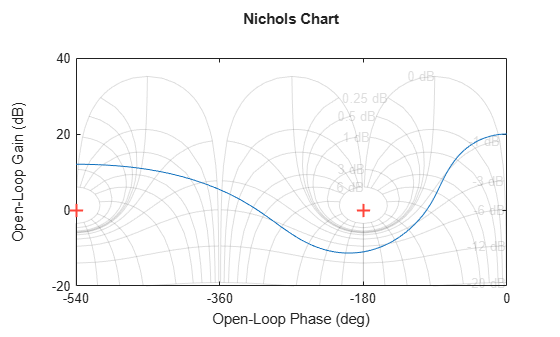
Represente la respuesta de Nichols con líneas de cuadrícula de Nichols para el siguiente sistema:

$$H(s)=\frac{-4s^4+48s^3-18s^2+250s+600}{s^4+30s^3+282s^2+525s+60}.$$

H = tf([-4 48 -18 250 600],[1 30 282 525 60]);
nichols(H)
grid

Gráfica de Nichols en frecuencias especificadas

Cree una gráfica de Nichols a lo largo de un rango de frecuencia especificado. Utilice este enfoque cuando desee centrarse en la dinámica de un rango de frecuencia en particular.

H = tf([-0.1,-2.4,-181,-1950],[1,3.3,990,2600]);
nichols(H,{1,100})

El arreglo de celdas {1,100} especifica el valor de frecuencia mínimo y máximo de la gráfica de Nichols. Cuando establece límites de frecuencia de esta manera, la función selecciona los puntos intermedios para los datos de respuesta en frecuencia.

Como alternativa, especifique un vector de puntos de frecuencia para utilizar cuando evalúe y represente la respuesta en frecuencia.

w = 1:0.5:100;
nichols(H,w,'.-')

nichols representa la respuesta en frecuencia solo en las frecuencias especificadas.

Gráfica de Nichols de varios sistemas dinámicos

Compare la respuesta en frecuencia de un sistema en tiempo continuo con un sistema discretizado equivalente en la misma gráfica de Nichols.

Cree sistemas dinámicos en tiempo continuo y tiempo discreto.

H = tf([1 0.1 7.5],[1 0.12 9 0 0]);
Hd = c2d(H,0.5,'zoh');

Cree una gráfica de Nichols que muestre ambos sistemas.

nichols(H,Hd)

Gráfica de Nichols con atributos de línea especificados

Especifique el estilo de línea, el color o el marcador en cada sistema de una gráfica de Nichols utilizando el argumento de entrada LineSpec.

H = tf([1 0.1 7.5],[1 0.12 9 0 0]);
Hd = c2d(H,0.5,'zoh');
nichols(H,'r',Hd,'b--')

La primera LineSpec, 'r', especifica una línea continua roja para la respuesta de H. La segunda LineSpec, 'b--', especifica una línea discontinua azul para la respuesta de Hd.

Datos de magnitud y fase de la respuesta de Nichols

Calcule la magnitud y la fase de la respuesta en frecuencia de un sistema SISO.

Si no se especifican frecuencias, nichols elige frecuencias en función de la dinámica del sistema y las devuelve en el tercer argumento de salida.

H = tf([1 0.1 7.5],[1 0.12 9 0 0]);
[mag,phase,wout] = nichols(H);

Dado que H es un modelo SISO, las primeras dos dimensiones de mag y phase son 1. La tercera dimensión es el número de frecuencias de wout.

size(mag)

ans = 1×3

     1     1   110

length(wout)

ans = 
110

De este modo, cada entrada a lo largo de la tercera dimensión de mag proporciona la magnitud de la respuesta en la correspondiente frecuencia de wout.

Gráfica de Nichols de un sistema MIMO

Para este ejemplo, cree un sistema de dos salidas y tres entradas.

rng(0,'twister');
H = rss(4,2,3);

En este sistema, nichols representa las respuestas en frecuencia de cada canal de E/S en un diagrama diferente y en una única figura.

nichols(H)

Calcule la magnitud y la fase de estas respuestas en 20 frecuencias entre 1 y 10 radianes.

w = logspace(0,1,20);
[mag,phase] = nichols(H,w);

mag y phase son arreglos tridimensionales en los que las primeras dos dimensiones corresponden a las dimensiones de salida y entrada de H y la tercera dimensión es el número de frecuencias. A modo de ejemplo, examine las dimensiones de mag.

size(mag)

ans = 1×3

     2     3    20

De este modo, por ejemplo, mag(1,3,10) es la magnitud de la respuesta desde la tercera entrada hasta la primera salida, calculada en la 10.ª frecuencia de w. Del mismo modo, phase(1,3,10) contiene la fase de la misma respuesta.

Gráfica de Nichols de un modelo con coeficientes complejos

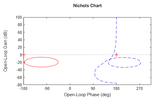
Cree una gráfica de Nichols de un modelo con coeficientes complejos y un modelo con coeficientes reales en el mismo diagrama.

rng(0)
A = [-3.50,-1.25-0.25i;2,0];
B = [1;0];
C = [-0.75-0.5i,0.625-0.125i];
D = 0.5;
Gc = ss(A,B,C,D);
Gr = rss(7);
nichols(Gc,Gr)
legend('Complex-coefficient model','Real-coefficient model','Location','southwest')

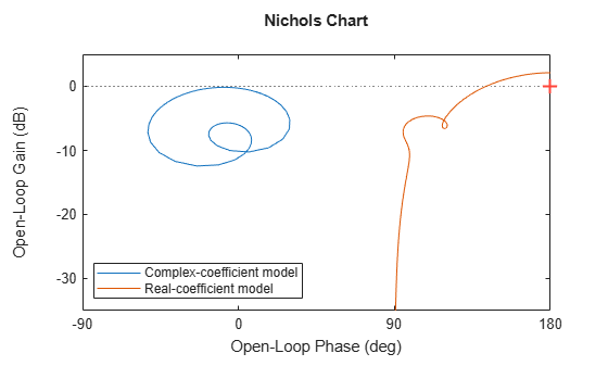
Para modelos con coeficientes complejos, nichols muestra un contorno que consta de frecuencias positivas y negativas. Para modelos con coeficientes reales, el diagrama muestra solo frecuencias positivas, incluso cuando hay modelos de coeficientes complejos. Puede hacer clic en la curva para examinar mejor qué sección y valores corresponden a frecuencias positivas y negativas.

Argumentos de entrada

sys — Sistema dinámico

modelo de sistema dinámico | arreglo de modelos

Sistema dinámico, especificado como un modelo de sistema dinámico SISO o MIMO, o bien un arreglo de modelos de sistemas dinámicos. Puede utilizar los siguientes tipos de sistemas dinámicos:

• Modelos LTI numéricos en tiempo continuo o en tiempo discreto, como modelos tf, zpk o ss.

• Modelos dispersos en espacio de estados, como modelos sparss o mechss. La cuadrícula de frecuencia w debe estar especificada para modelos dispersos.

• Modelos LTI generalizados o con incertidumbre, como modelos genss o uss (Robust Control Toolbox). El uso de modelos con incertidumbre requiere Robust Control Toolbox™.

  • En el caso de bloques de diseño de control ajustables, la función evalúa el modelo con su valor actual para representar la respuesta.

  • En el caso de los bloques de diseño de control con incertidumbre, la función representa el valor nominal y muestras aleatorias del modelo.

• Modelos de datos de respuesta en frecuencia, como modelos frd. Para estos modelos, la función representa la respuesta en las frecuencias definidas en el modelo.

• Modelos LTI identificados, como modelos idtf (System Identification Toolbox), idss (System Identification Toolbox) o idproc (System Identification Toolbox). El uso de modelos identificados requiere System Identification Toolbox™.

Si sys es un arreglo de modelos, la gráfica muestra las respuestas de todos los modelos del arreglo en los mismos ejes.

w — Frecuencias

{wmin,wmax} | vector | []

Frecuencias en las que calcular y representar la respuesta en frecuencia, especificadas como el arreglo de celdas {wmin,wmax} o como un vector de valores de frecuencia.

• Si w es un arreglo de celdas en formato {wmin,wmax}, entonces la función calcula la respuesta en frecuencias entre wmin y wmax.

• Si w es un vector de frecuencias, entonces la función calcula la respuesta en cada frecuencia especificada. Por ejemplo, utilice logspace para generar un vector fila con valores de frecuencia espaciados logarítmicamente. El vector w puede contener frecuencias positivas y negativas.

• []: selecciona automáticamente las frecuencias en función de la dinámica del sistema.

Para modelos con coeficientes complejos, si especifica un rango de frecuencia de [w_min,w_max] para su gráfica, la gráfica muestra un contorno formado tanto por frecuencias positivas [w_min,w_max] como por frecuencias negativas [–w_max,–w_min].

Especifique frecuencias en unidades de rad/TimeUnit, donde TimeUnit es la propiedad TimeUnit del modelo.

Argumentos de salida

mag — Magnitud de la respuesta del sistema

arreglo 3D

Magnitud de la respuesta del sistema en unidades absolutas, devuelta como un arreglo 3D. Las dimensiones de este arreglo son (número de salidas del sistema) × (número de entradas del sistema) × (número de puntos de frecuencia).

• En los sistemas SISO, mag(1,1,k) proporciona la magnitud de la respuesta en la k-ésima frecuencia de w o wout. Para ver un ejemplo, consulte Datos de magnitud y fase de la respuesta de Nichols.

• En los sistemas MIMO, mag(i,j,k) proporciona la magnitud de la respuesta en la k-ésima frecuencia desde la j-ésima entrada hasta la i-ésima salida. Para ver un ejemplo, consulte Gráfica de Nichols de un sistema MIMO.

Para convertir la magnitud de unidades absolutas a decibelios, utilice:

magdb = 20*log10(mag)

phase — Fase de la respuesta del sistema

arreglo 3D

Fase de la respuesta del sistema en grados, devuelta como un arreglo 3D. Las dimensiones de este arreglo son (número de salidas) por (número de entradas) por (número de puntos de frecuencia).

• En los sistemas SISO, phase(1,1,k) proporciona la fase de la respuesta en la k-ésima frecuencia de w o wout. Para ver un ejemplo, consulte Datos de magnitud y fase de la respuesta de Nichols.

• En los sistemas MIMO, phase(i,j,k) proporciona la fase de la respuesta en la k-ésima frecuencia desde la j-ésima entrada hasta la i-ésima salida. Para ver un ejemplo, consulte Gráfica de Nichols de un sistema MIMO.

wout — Frecuencias

vector

Frecuencias en las que la función devuelve la respuesta del sistema, devueltas como un vector columna. La función elige los valores de frecuencia en función de la dinámica del modelo, a menos que especifique frecuencias con el argumento de entrada w.

wout también contiene valores de frecuencia negativos para modelos con coeficientes complejos.

Los valores de frecuencia se expresan en radianes/TimeUnit, donde TimeUnit es el valor de la propiedad TimeUnit de sys.

Sugerencias

• Cuando necesite opciones de personalización de gráficas adicionales, utilice en su lugar nicholsplot.

• Las gráficas creadas con nichols no admiten títulos ni etiquetas multilínea especificados como arreglos de cadenas o arreglos de celdas de vectores de caracteres. Para especificar títulos y etiquetas multilínea, utilice una cadena única con un carácter newline.

  nichols(sys)
  title("first line" + newline + "second line");

Historial de versiones

Introducido antes de R2006a

R2024b: gca ahora devuelve un objeto de gráfico

En el caso de gráficas creadas con nichols, la función gca ahora devuelve un objeto de gráfico nicholsplot en lugar de un eje dentro de la gráfica.

Consulte también

nyquist | bode | nicholsplot

Temas

• Respuestas en el dominio de la frecuencia
• Modelos de sistemas dinámicos