Data Sets for Deep Learning
Use these data sets to get started with deep learning applications.
Note
Some of the code used in these data set descriptions use functions attached to examples as supporting files. To use these functions, open the examples as live scripts.
Image Data Sets
| Data Set | Description | Task |
|---|---|---|
Digits
| The Digits data set consists of 10,000 synthetic grayscale images of handwritten digits. Each image is 28-by-28 pixels and has an associated label denoting which digit the image represents (0–9). Each image has been rotated by a certain angle. When loading the images as arrays, you can also load the rotation angle of the image. Load the Digits data as in-memory numeric arrays
using the [XTrain,YTrain,anglesTrain] = digitTrain4DArrayData; [XTest,YTest,anglesTest] = digitTest4DArrayData; For examples showing how to process this data for deep learning, see Monitor Deep Learning Training Progress and Train Convolutional Neural Network for Regression. | Image classification and image regression |
Load the Digits data as an image datastore using the unzip("DigitsData.zip"); dataFolder = "DigitsData"; imds = imageDatastore(dataFolder, ... IncludeSubfolders=true, ... LabelSource="foldernames"); For an example showing how to process this data for deep learning, see Create Simple Deep Learning Neural Network for Classification. | Image classification | |
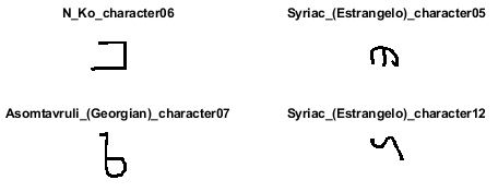
Omniglot
| The Omniglot data set contains character sets for 50 alphabets, divided into 30 sets for training and 20 sets for testing [1]. Each alphabet contains a number of characters, from 14 for Ojibwe (Canadian Aboriginal syllabics) to 55 for Tifinagh. Finally, each character has 20 handwritten observations. Download and
extract the Omniglot data set from https://github.com/brendenlake/omniglot. Set
downloadFolder = tempdir;

url = "https://github.com/brendenlake/omniglot/raw/master/python";

urlTrain = url + "/images_background.zip";
urlTest = url + "/images_evaluation.zip";

filenameTrain = fullfile(downloadFolder,"images_background.zip");
filenameTest = fullfile(downloadFolder,"images_evaluation.zip");

dataFolderTrain = fullfile(downloadFolder,"images_background");
dataFolderTest = fullfile(downloadFolder,"images_evaluation");

if ~exist(dataFolderTrain,"dir")
    fprintf("Downloading Omniglot training data set (4.5 MB)... ")
    websave(filenameTrain,urlTrain);
    unzip(filenameTrain,downloadFolder);
    fprintf("Done.\n")
end

if ~exist(dataFolderTest,"dir")
    fprintf("Downloading Omniglot test data (3.2 MB)... ")
    websave(filenameTest,urlTest);
    unzip(filenameTest,downloadFolder);
    fprintf("Done.\n")
end
To
load the training and test data as image datastores, use the
imdsTrain = imageDatastore(dataFolderTrain, ...
    'IncludeSubfolders',true, ...
    'LabelSource','none');

files = imdsTrain.Files;
parts = split(files,filesep);
labels = join(parts(:,(end-2):(end-1)),'_');
imdsTrain.Labels = categorical(labels);

imdsTest = imageDatastore(dataFolderTest, ...
    'IncludeSubfolders',true, ...
    'LabelSource','none');

files = imdsTest.Files;
parts = split(files,filesep);
labels = join(parts(:,(end-2):(end-1)),'_');
imdsTest.Labels = categorical(labels);
For an example showing how to process this data for deep learning, see Train a Twin Neural Network to Compare Images. | Image similarity |
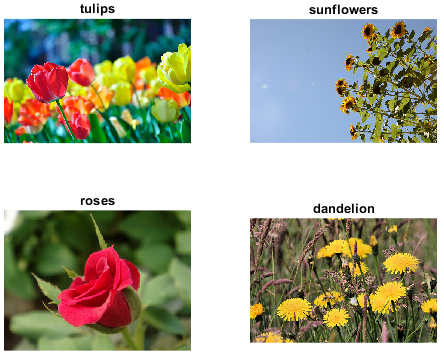
Flowers
| The Flowers data set contains 3670 images of flowers belonging to five classes (daisy, dandelion, roses, sunflowers, and tulips) [2]. Download and extract the Flowers data set from http://download.tensorflow.org/example_images/flower_photos.tgz. The data set is about 218 MB. Set
url = 'http://download.tensorflow.org/example_images/flower_photos.tgz';
downloadFolder = tempdir;
filename = fullfile(downloadFolder,'flower_dataset.tgz');

dataFolder = fullfile(downloadFolder,'flower_photos');
if ~exist(dataFolder,'dir')
    fprintf("Downloading Flowers data set (218 MB)... ")
    websave(filename,url);
    untar(filename,downloadFolder)
    fprintf("Done.\n")
end
Load
the data as an image datastore using the
imds = imageDatastore(dataFolder, ...
    'IncludeSubfolders',true, ...
    'LabelSource','foldernames');
For an example showing how to process this data for deep learning, see Train Generative Adversarial Network (GAN). | Image classification |
Example Food Images
| The Example Food Images data set contains 978 photographs of food in nine classes (caesar_salad, caprese_salad, french_fries, greek_salad, hamburger, hot_dog, pizza, sashimi, and sushi). Download the Example
Food Images data set using the
fprintf("Downloading Example Food Image data set (77 MB)... ")
filename = matlab.internal.examples.downloadSupportFile('nnet', ...
    'data/ExampleFoodImageDataset.zip');
fprintf("Done.\n")

filepath = fileparts(filename);
dataFolder = fullfile(filepath,'ExampleFoodImageDataset');
unzip(filename,dataFolder);
For an example showing how to process this data for deep learning, see View Network Behavior Using tsne. | Image classification |
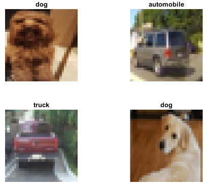
CIFAR-10
(Representative example) | The CIFAR-10 data set contains 60,000 color images of size 32-by-32 pixels, belonging to 10 classes (airplane, automobile, bird, cat, deer, dog, frog, horse, ship, and truck) [7]. There are 6,000 images per class. The data set is split into a training set with 50,000 images and a test set with 10,000 images. This data set is one of the most widely used data sets for testing new image classification models. Download and extract the CIFAR-10 data set from https://www.cs.toronto.edu/%7Ekriz/cifar-10-matlab.tar.gz. The data set is about 175 MB. Set
url = 'https://www.cs.toronto.edu/~kriz/cifar-10-matlab.tar.gz'; downloadFolder = tempdir; filename = fullfile(downloadFolder,'cifar-10-matlab.tar.gz'); dataFolder = fullfile(downloadFolder,'cifar-10-batches-mat'); if ~exist(dataFolder,'dir') disp("Downloading CIFAR-10 dataset (175 MB)... "); websave(filename,url); untar(filename,downloadFolder); disp("Done.") end loadCIFARData, which is used in
the example Train Residual Network for Image Classification.
To access this function, open the example as a live
script.[XTrain,YTrain,XValidation,YValidation] = loadCIFARData(downloadFolder); For an example showing how to process this data for deep learning, see Train Residual Network for Image Classification. | Image classification |
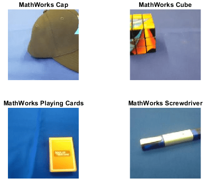
MathWorks® Merch
| The MathWorks Merch data set is a small data set containing 75 images of MathWorks merchandise, belonging to five different classes (cap, cube, playing cards, screwdriver, and torch). You can use this data set to try out transfer learning and image classification quickly. The images are of size 227-by-227-by-3. Extract the MathWorks Merch data set. filename = 'MerchData.zip'; dataFolder = fullfile(tempdir,'MerchData'); if ~exist(dataFolder,'dir') unzip(filename,tempdir); end Load the data as an image datastore
using the imds = imageDatastore(dataFolder, ... 'IncludeSubfolders',true,'LabelSource','foldernames'); For examples showing how to process this data for deep learning, see Get Started with Transfer Learning and Retrain Neural Network to Classify New Images. | Image classification |
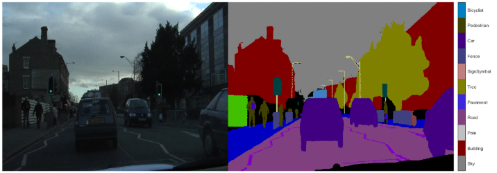
CamVid
| The CamVid data set is a collection of images containing street-level views obtained from cars being driven [8]. The data set is useful for training networks that perform semantic segmentation of images and provides pixel-level labels for 32 semantic classes, including car, pedestrian, and road. The images are of size 720-by-960-by-3. Download and extract the CamVid data
set from http://web4.cs.ucl.ac.uk/staff/g.brostow/MotionSegRecData/. The data set is about 573 MB. Set
downloadFolder = tempdir;
url = "http://web4.cs.ucl.ac.uk/staff/g.brostow/MotionSegRecData"
urlImages = url + "/files/701_StillsRaw_full.zip";
urlLabels = url + "/data/LabeledApproved_full.zip";

dataFolder = fullfile(downloadFolder,"CamVid");
dataFolderImages = fullfile(dataFolder,"images");
dataFolderLabels = fullfile(dataFolder,"labels");

filenameLabels = fullfile(dataFolder,"labels.zip");
filenameImages = fullfile(dataFolder,"images.zip");

if ~exist(filenameLabels,"file") || ~exist(imagesZip,"file")
    mkdir(dataFolder)

    disp("Downloading CamVid data set images (557 MB)... ");
    websave(filenameImages, urlImages);
    unzip(filenameImages,dataFolderImages);
    disp("Done.")

    disp("Downloading CamVid data set labels (16 MB)... ");
    websave(filenameLabels,urlLabels);
    unzip(filenameLabels,dataFolderLabels);
    disp("Done.")
end
Load the data as a pixel label
datastore using the imds = imageDatastore(dataFolderImages,"IncludeSubfolders",true); classes = ["Sky" "Building" "Pole" "Road" "Pavement" "Tree" ... "SignSymbol" "Fence" "Car" "Pedestrian" "Bicyclist"]; labelIDs = camvidPixelLabelIDs; pxds = pixelLabelDatastore(dataFolderLabels,classes,labelIDs); For an example showing how to process this data for deep learning, see Semantic Segmentation Using Deep Learning (Computer Vision Toolbox). | Semantic segmentation |
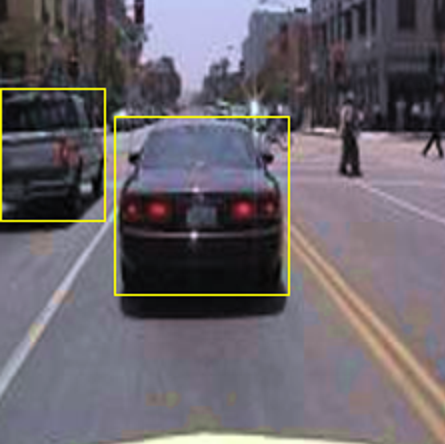
Vehicle
| The Vehicle data set consists of 295 images containing one or two labeled instances of a vehicle. This small data set is useful for exploring the YOLO training procedure, but in practice, more labeled images are needed to train a robust detector. The images are of size 720-by-960-by-3. Extract the Vehicle data set. Set
filename = "vehicleDatasetImages.zip";

dataFolder = fullfile(tempdir,"vehicleImages");
if ~exist(dataFolder,"dir")
    unzip(filename,tempdir);
end
Load the data set as a table of file names and bounding boxes from the extracted MAT file and convert the file names to absolute file paths. data = load("vehicleDatasetGroundTruth.mat");
vehicleDataset = data.vehicleDataset;
vehicleDataset.imageFilename = fullfile(tempdir,vehicleDataset.imageFilename);Create
an image datastore containing the images and a box label datastore
containing the bounding boxes using the
filenamesImages = vehicleDataset.imageFilename;
tblBoxes = vehicleDataset(:,"vehicle");

imds = imageDatastore(filenamesImages);
blds = boxLabelDatastore(tblBoxes);

cds = combine(imds,blds);
For an example showing how to process this data for deep learning, see Object Detection Using YOLO v4 Deep Learning (Computer Vision Toolbox). | Object detection |
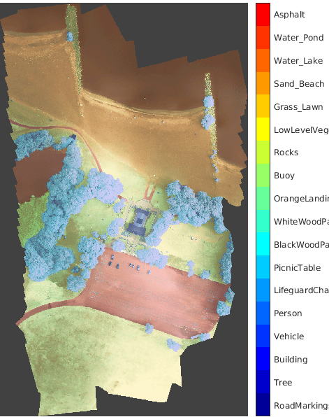
RIT-18
| The RIT-18 data set contains image data captured by a drone over Hamlin Beach State Park in New York state [9]. The data contains labeled training, validation, and test sets, with 18 object class labels including road markings, tree, and building. The data set is about 3 GB. Download the RIT-18 data set from https://home.cis.rit.edu/~cnspci/other/data/rit18_data.mat. Set downloadFolder = tempdir; url = "https://home.cis.rit.edu/~cnspci/other/data/rit18_data.mat"; filename = fullfile(downloadFolder,"rit18_data.mat"); if ~exist(filename,"file") disp("Downloading Hamlin Beach data set (3 GB)... "); websave(filename,url); disp("Done.") end For an example showing how to process this data for deep learning, see Semantic Segmentation of Multispectral Images Using Deep Learning (Image Processing Toolbox). | Semantic segmentation |
BraTS
| The BraTS data set contains MRI scans of brain tumors, namely gliomas, which are the most common primary brain malignancies [10]. The data set contains 750 4-D volumes, each representing a stack of 3-D images. Each 4-D volume is of size 240-by-240-by-155-by-4, where the first three dimensions correspond to the height, width, and depth of a 3-D volumetric image. The fourth dimension corresponds to different scan modalities. The data set is divided into 484 training volumes with voxel labels and 266 test volumes. The data set is about 7 GB. Create a directory to store the BraTS data set. dataFolder = fullfile(tempdir,"BraTS"); if ~exist(dataFolder,"dir") mkdir(dataFolder); end Download the BraTS data from Medical Segmentation Decathlon by clicking the "Download Data" link. Download the "Task01_BrainTumour.tar" file. Extract the TAR file into
the directory specified by the For an example showing how to process this data for deep learning, see 3-D Brain Tumor Segmentation Using Deep Learning (Image Processing Toolbox). | Semantic segmentation |
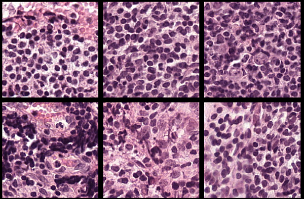
Camelyon16
| The data from the Camelyon16 challenge contains a total of 400 whole-slide images (WSIs) of lymph nodes from two independent sources, separated into 270 training images and 130 test images [11]. The data set has a size of about 451 GB. The training data set consists of 159 WSIs of normal lymph nodes and 111 WSIs of lymph nodes with tumor and healthy tissue. Usually, the tumor tissue is a small fraction of the healthy tissue. Ground truth coordinates of the lesion boundaries accompany the tumor images. Create folders to store the Camelyon16 training data set on your local machine. dataDir = fullfile(tempdir,"Camelyon16","training"); trainNormalDir = fullfile(dataDir,"normal"); trainTumorDir = fullfile(dataDir,"tumor"); trainAnnotationDir = fullfile(dataDir,"lesion_annotations"); if ~exist(dataDir,"dir") mkdir(dataDir); mkdir(trainNormalDir); mkdir(trainTumorDir); mkdir(trainAnnotationDir); end To download the data, go to the GigaDB website for the data set, and, in the table, navigate to the Files tab. Download individual files by clicking on the name in the File Name column, and move them to the correct subfolders by following these steps:
For an example that shows how to process this data for deep learning, see Preprocess Multiresolution Images for Training Classification Network (Image Processing Toolbox). | Image classification (large images) |
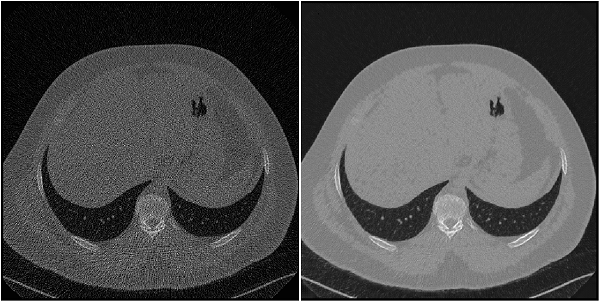
Low Dose CT Grand Challenge
| The Low Dose CT Grand Challenge includes pairs of regular-dose CT images and simulated low-dose CT images for 99 head scans (labeled N for neuro), 100 chest scans (labeled C for chest), and 100 abdomen scans (labeled L for liver) [12] [13]. The full data set is about 1.2 TB. Create a directory to store the chest files from the Low Dose CT Grand Challenge data set.
dataDir = fullfile(tempdir,"LDCT","LDCT-and-Projection-data");
if ~exist(dataDir,"dir")
    mkdir(dataDir);
end
To download the data, go to The Cancer Imaging Archive website. Download the chest
files from the "Images (DICOM, 952 GB)" data set using the NBIA Data Retriever. Specify the
For an example showing how to process this data for deep learning, see Unsupervised Medical Image Denoising Using CycleGAN (Image Processing Toolbox). | Image-to-image regression |
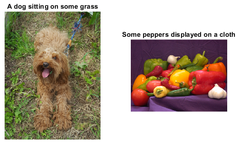
Common Objects in Context (COCO)
(Representative example) | The COCO 2014 train images data set consists of 82,783 images. The annotations data contains at least five captions corresponding to each image. Create directories to store the COCO data set. dataFolder = fullfile(tempdir,"coco"); if ~exist(dataFolder,"dir") mkdir(dataFolder); end Download
and extract the COCO 2014 train images and captions from https://cocodataset.org/#download by clicking the
"2014 Train images" and "2014 Train/Val annotations" links,
respectively. Save the data in the folder specified by
Extract the captions
from the file filename = fullfile(dataFolder,"annotations_trainval2014","annotations", ... "captions_train2014.json"); str = fileread(filename); data = jsondecode(str); The
For an example showing how to process this data for deep learning, see Image Captioning Using Attention. | Image captioning |
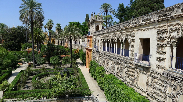
IAPR TC-12
(Representative example) | The IAPR TC-12 Benchmark consists of 20,000 still natural images [14]. The data set includes photos of people, animals, cities, and more. The data file is about 1.8 GB. Download the IAPR TC-12 data set. dataDir = fullfile(tempdir,"iaprtc12"); url = "https://www-i6.informatik.rwth-aachen.de/imageclef/resources/iaprtc12.tgz"; if ~exist(dataDir,"dir") disp("Downloading IAPR TC-12 data set (1.8 GB)..."); try untar(url,dataDir); catch % On some Windows machines, the untar command throws an error for .tgz % files. Rename to .tg and try again. fileName = fullfile(tempdir,"iaprtc12.tg"); websave(fileName,url); untar(fileName,dataDir); end disp("Done."); end Load the data as an image datastore using the imageDir = fullfile(dataDir,"images") exts = {".jpg",".bmp",".png"}; imds = imageDatastore(imageDir, ... "IncludeSubfolders",true,"FileExtensions",exts); For an example showing how to process this data for deep learning, see Increase Image Resolution Using Deep Learning (Image Processing Toolbox). | Image-to-image regression |
Zurich RAW to RGB
| The Zurich RAW to RGB data set contains 48,043 spatially registered pairs of RAW and RGB training image patches of size 448-by-448 [15]. The data set contains two separate test sets. One test set consists of 1,204 spatially registered pairs of RAW and RGB image patches of size 448-by-448. The other test set consists of unregistered full-resolution RAW and RGB images. The data set is 22 GB. Create a directory to store the Zurich RAW to RGB data set. dataDir = fullfile(tempdir,"ZurichRAWToRGB");dataDir variable. If the extraction is
successful, then dataDir contains three
directories: full_resolution,
test, and
train.For an example showing how to process this data for deep learning, see Develop Camera Processing Pipeline Using Deep Learning (Image Processing Toolbox). | Image-to-image regression |
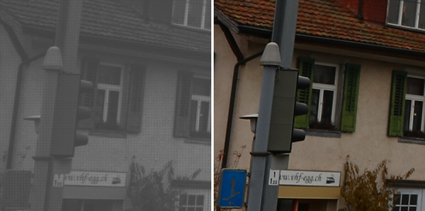
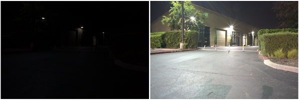
See-In-The-Dark (SID)
| The See-In-The-Dark (SID) data set provides registered pairs of RAW images of the same scene [16]. In each pair, one image has a short exposure time and is underexposed, and the other image has a longer exposure time and is well-exposed. The size of the Sony camera data from the SID data set is 25 GB. Specify dataDir = fullfile(tempdir,"SID"); if ~exist(dataDir,"dir") mkdir(dataDir); end To download the data set, go to
this link: https://storage.googleapis.com/isl-datasets/SID/Sony2025.zip. Extract the data into the directory specified by the
The data set also provides text files that
describe how to partition the files into training, validation, and
test data sets. Move the files "Sony_train_list.txt",
"Sony_val_list.txt", and "Sony_test_list.txt" to the directory
specified by the For an example showing how to process this data for deep learning, see Brighten Extremely Dark Images Using Deep Learning (Image Processing Toolbox). | Image-to-image regression |
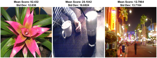
LIVE In the Wild
| The LIVE In the Wild data set consists of 1,162 photos captured by mobile devices, with seven additional training images [17]. Each image is rated by an average of 175 individuals on a scale of [1, 100]. The data set provides the mean and standard deviation of the subjective scores for each image. Specify
imageDir = fullfile(tempdir,"LIVEInTheWild");
if ~exist(imageDir,"dir")
    mkdir(imageDir);
end
Download the data set by following the
instructions outlined in LIVE In the Wild Image Quality Challenge Database.
Extract the data into the directory specified by the
For an example showing how to process this data for deep learning, see Quantify Image Quality Using Neural Image Assessment (Image Processing Toolbox). | Image classification |
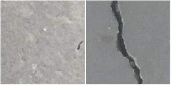
Concrete Crack Images for Classification
| The Concrete Crack Images for Classification data set contains images of two classes: "Negative" images without cracks present in the road and "Positive" images with cracks [18] [19]. The data set provides 20,000 images of each class. The size of the data set is about 230 MB. Specify
dataDir = fullfile(tempdir,"ConcreteCracks");
if ~exist(dataDir,"dir")
    mkdir(dataDir);
end
To download the data set, go to this link:
Concrete Crack Images for Classification. Extract the
downloaded ZIP file to obtain a RAR file, then extract the contents
of the RAR file into the directory specified by the
For an example showing how to process this data for deep learning, see Detect Image Anomalies Using Pretrained ResNet-18 Feature Embeddings (Computer Vision Toolbox). | Image classification |
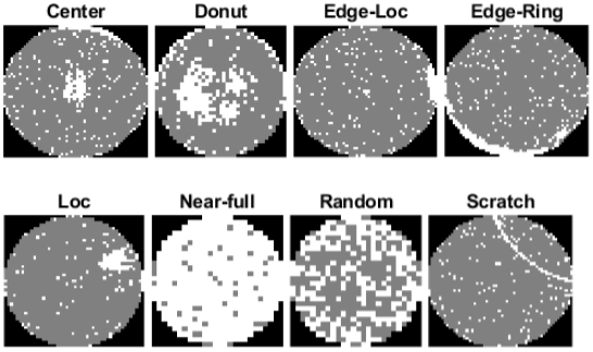
MIR WM-811K (Wafer Defect Maps)
| The Wafer Defect Map data set consists of 811,457 wafer map images, including 172,950 labeled images [20] [21]. Each image has only three pixel values. The value 0 indicates the background, the value 1 represents correctly behaving dies, and the value 2 represents defective dies. The labeled images have one of nine labels based on the spatial pattern of defects. The size of the data set is 3.5 GB. Specify
dataDir = fullfile(tempdir,"WaferDefects");
dataURL = "http://mirlab.org/dataSet/public/MIR-WM811K.zip";
dataMatFile = fullfile(dataDir,"MIR-WM811K","MATLAB","WM811K.mat");

if exist(dataMatFile,"file") ~= 2
    unzip(dataURL,dataDir);
end
The data is stored in a MAT file as an array of structures. Load the data set into the workspace. waferData = load(dataMatFile); waferData = waferData.data; For an example showing how to process this data for deep learning, see Classify Defects on Wafer Maps Using Deep Learning (Computer Vision Toolbox). | Image classification |
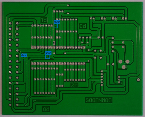
PCB Defect
| The Printed Circuit Board (PCB) Defect data set contains 1,386 images of PCB elements with synthesized defects [22] [23]. The data has six types of defects: missing hole, mouse bite, open circuit, short, spur, and spurious copper. Each image contains multiple defects of the same category in different locations. The data set provides bounding box and coordinate information for every defect in every image. The size of the data set is 1.87 GB. Specify dataDir = fullfile(tempdir,"PCBDefects"); imageDir = fullfile(dataDir,"PCB-DATASET-master"); if ~exist(imageDir,"dir") dataURL = "https://github.com/Ironbrotherstyle/PCB-DATASET/archive/refs/heads/master.zip"; unzip(dataURL,dataDir); delete(fullfile(imageDir,"*.m"),fullfile(imageDir,"*.mlx"), ... fullfile(imageDir,"*.mat"),fullfile(imageDir,"*.md")); end For an example showing how to process this data for deep learning, see Detect Defects on Printed Circuit Boards Using YOLOX Network (Computer Vision Toolbox). | Object detection |
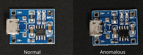
Visual Anomaly (VisA)
| The Visual Anomaly (VisA) data set consists of 10,821 high-resolution color images (9,621 normal and 1,200 anomalous samples) covering 12 different object subsets in three domains [24][25]. Four of the subsets correspond to four different types of PCBs, containing transistors, capacitors, chips, and other components. The anomalous images in the test set contain various surface defects (such as scratches, dents, color spots or cracks), and structural defects (such as part misplacement or missing parts). The data set contains 5 to 20 images per defect type and some images contain multiple defects. Download one of the four PCB data
subsets for deep learning. This data subset contains
Specify imageDir = fullfile(tempdir,"VisA"); if ~exist(imageDir,"dir") dataURL = "https://ssd.mathworks.com/supportfiles/vision/data/VisA.zip"; unzip(dataURL,dataDir); delete(fullfile(imageDir,"*.m"),fullfile(imageDir,"*.mlx"), ... fullfile(imageDir,"*.mat"),fullfile(imageDir,"*.md")); end For an example that shows how to process this data for deep learning, see Localize Industrial Defects Using PatchCore Anomaly Detector (Computer Vision Toolbox). | Image classification |
Pill Quality Control (Pill QC)
| The Pill QC data set contains images of three classes: "normal" images without defects, "chip" images with chip defects in the pills, and "dirt" images with dirt contamination. The data set provides 149 normal images, 43 chip images, and 138 dirt images. The size of the data set is 3.57 MB. Specify
dataDir = fullfile(tempdir,"PillDefects");
imageDir = fullfile(dataDir,"pillQC-main");

if ~exist(imageDir,"dir")
    unzip("https://github.com/matlab-deep-learning/pillQC/archive/refs/heads/main.zip",dataDir);
end
Load
the data as an image datastore using the
imageDir = fullfile(dataDir,"pillQC-main","images");
imds = imageDatastore(imageDir,IncludeSubfolders=true,LabelSource="foldernames");
For an example showing how to process this data for deep learning, see Detect Image Anomalies Using Explainable FCDD Network (Computer Vision Toolbox). | Image classification |
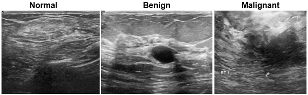
Breast Ultrasound Images (BUSI)
| The Breast Ultrasound Images (BUSI) data set contains 2-D breast ultrasound images [26]. The data set contains 133 normal images, 487 images with benign tumors, and 210 images with malignant tumors. Each ultrasound image has a corresponding tumor mask image for training semantic segmentation networks. The tumor mask labels have been reviewed by clinical radiologists. The size of the data set is approximately 197 MB. Download the BUSI data set from the MathWorks website. zipFile = matlab.internal.examples.downloadSupportFile("image","data/Dataset_BUSI.zip"); filepath = fileparts(zipFile); unzip(zipFile,filepath) Load the data as an
image datastore using the imageDir = fullfile(filepath,"Dataset_BUSI_with_GT"); imds = imageDatastore(imageDir,IncludeSubfolders=true,LabelSource="foldernames"); For an example showing how to process this data for deep learning, see Breast Tumor Segmentation from Ultrasound Using Deep Learning (Medical Imaging Toolbox). | Semantic segmentation |
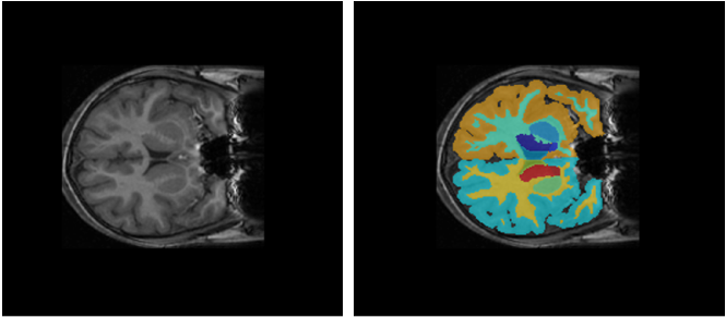
Child and Adolescent NeuroDevelopment Initiative (CANDI) neuroimaging data set
| The CANDI data set (subset HC_001) contains one brain MRI image volume and its corresponding segmentation label image [27]. The total size of the data set is approximately 2.5 MB. Download the CANDI data set from the MathWorks website. zipFile = matlab.internal.examples.downloadSupportFile("image","data/brainSegData.zip"); filepath = fileparts(zipFile); unzip(zipFile,filepath) dataDir = fullfile(filepath,"brainSegData"); For an example showing how to load and process this data for deep learning, see Brain MRI Segmentation Using Pretrained 3-D U-Net Network (Medical Imaging Toolbox) | Semantic segmentation |
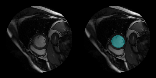
Sunnybrook Cardiac Data set
| The Sunnybrook Cardiac Data set contains cine MRI images and ground truth labels of the left ventricle [28]. The data set contains images from multiple patients with various cardiac pathologies. The MRI images are in the DICOM file format and the label images are in the PNG file format. This code downloads a subset of the original data set from the MathWorks website. The subset contains MRI images and label images from 45 patients. The total download size is approximately 105 MB. zipFile = matlab.internal.examples.downloadSupportFile("medical","CardiacMRI.zip"); filepath = fileparts(zipFile); unzip(zipFile,filepath) The
imageDir = fullfile(filepath,"Cardiac MRI");
For an example showing how to process this data for deep learning, see Cardiac Left Ventricle Segmentation from Cine-MRI Images Using U-Net Network (Medical Imaging Toolbox). | Semantic segmentation |


Time Series and Signal Data Sets
| Data | Description | Task |
|---|---|---|
Japanese Vowels
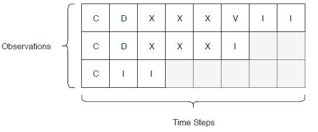
| The Japanese Vowels data set contains preprocessed sequences representing utterances of Japanese vowels from different speakers [29] [30].
Load the
Japanese Vowels training and test data sets as in-memory cell arrays
containing numeric sequences using load JapaneseVowelsTrainData load JapaneseVowelsTestData For an example showing how to process this data for deep learning, see Sequence Classification Using Deep Learning. | Sequence-to-label classification |
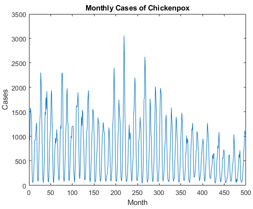
Chickenpox
| The Chickenpox data set contains a single time series, with time steps corresponding to months and values corresponding to the number of cases. The output is a cell array, where each element is a single time step. Load the Chickenpox data as a single
numeric sequences using the data = chickenpox_dataset;
data = [data{:}]'; | Time-series forecasting |
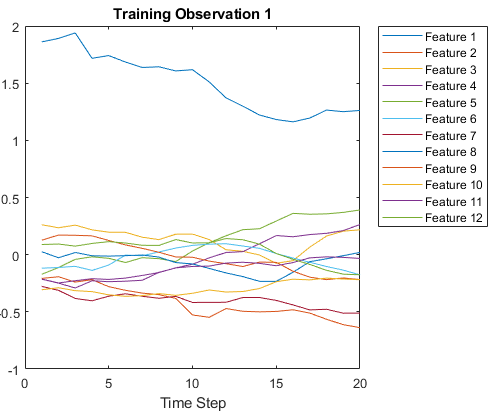
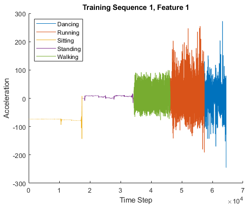
Human Activity
| The Human Activity data set contains seven time series of sensor data obtained from a smartphone worn on the body. Each sequence has three features and varies in length. The three features correspond to accelerometer readings in three different directions. Load the Human Activity data set. dataTrain = load('HumanActivityTrain'); dataTest = load('HumanActivityTest'); XTrain = dataTrain.XTrain; YTrain = dataTrain.YTrain; XTest = dataTest.XTest; YTest = dataTest.YTest; For an example showing how to process this data for deep learning, see Sequence-to-Sequence Classification Using Deep Learning. | Sequence-to-sequence classification |
Turbofan Engine Degradation Simulation
| Each time series of the Turbofan Engine Degradation Simulation data set represents a different engine [31]. Each engine starts with unknown degrees of initial wear and manufacturing variation. The engine is operating normally at the start of each time series, and develops a fault at some point during the series. In the training set, the fault grows in magnitude until system failure. The data contains a ZIP-compressed text files with 26 columns of numbers, separated by spaces. Each row is a snapshot of data taken during a single operational cycle, and each column is a different variable. The columns correspond to the following:
Create a directory to store the Turbofan Engine Degradation Simulation data set. dataFolder = fullfile(tempdir,"turbofan"); if ~exist(dataFolder,'dir') mkdir(dataFolder); end Download and extract the Turbofan Engine Degradation Simulation data set. filename = matlab.internal.examples.downloadSupportFile( ... "nnet","data/TurbofanEngineDegradationSimulationData.zip"); unzip(filename,dataFolder) Load
the training and test data using the helper functions
filenamePredictors = fullfile(dataFolder,"train_FD001.txt");
[XTrain,YTrain] = processTurboFanDataTrain(filenamePredictors);

filenamePredictors = fullfile(dataFolder,"test_FD001.txt");
filenameResponses = fullfile(dataFolder,"RUL_FD001.txt");
[XTest,YTest] = processTurboFanDataTest(filenamePredictors,filenameResponses);
For an example showing how to process this data for deep learning, see Sequence-to-Sequence Regression Using Deep Learning. | Sequence-to-sequence regression, predictive maintenance |
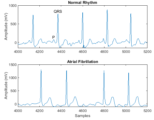
PhysioNet 2017 Challenge
| The PhysioNet 2017 Challenge data set consists of a set of electrocardiogram (ECG) recordings sampled at 300 Hz and divided by a group of experts into different classes [33]. Download and extract the PhysioNet 2017 Challenge
data set using the ReadPhysionetData
data = load('PhysionetData.mat')
signals = data.Signals;
labels = data.Labels;For an example showing how to process this data for deep learning, see Classify ECG Signals Using Long Short-Term Memory Networks. | Sequence-to-label classification |
Tennessee Eastman Process (TEP) simulation
| This data set consists of MAT files converted from the Tennessee Eastman Process (TEP) simulation data [32]. Download the Tennessee Eastman Process (TEP) simulation data set from the MathWorks support files site (see disclaimer). The data set has four components: fault-free training, fault-free testing, faulty training, and faulty testing. Download each file separately. The data set is 1.7 GB. fprintf("Downloading TEP faulty training data (613 MB)... ") filenameFaultyTrain = matlab.internal.examples.downloadSupportFile('predmaint', ... 'chemical-process-fault-detection-data/faultytraining.mat'); fprintf("Done.\n") fprintf("Downloading TEP faulty testing data (1 GB)... ") filenameFaultyTest = matlab.internal.examples.downloadSupportFile('predmaint', ... 'chemical-process-fault-detection-data/faultytesting.mat'); fprintf("Done.\n") fprintf("Downloading TEP fault-free training data (36 MB)... ") filenameFaultFreeTrain = matlab.internal.examples.downloadSupportFile('predmaint', ... 'chemical-process-fault-detection-data/faultfreetraining.mat'); fprintf("Done.\n") fprintf("Downloading TEP fault-free testing data (69 MB)... ") filenameFaultFreeTest = matlab.internal.examples.downloadSupportFile('predmaint', ... 'chemical-process-fault-detection-data/faultfreetesting.mat'); fprintf("Done.\n") Load the downloaded files into the MATLAB® workspace. load(filenameFaultyTrain); load(filenameFaultyTest); load(filenameFaultFreeTrain); load(filenameFaultFreeTest); For an example showing how to process this data for deep learning, see Chemical Process Fault Detection Using Deep Learning. | Sequence-to-label classification |
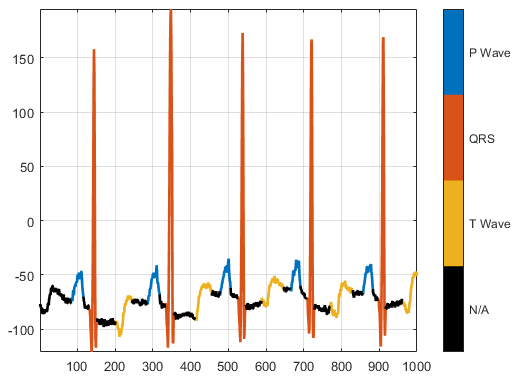
PhysioNet ECG Segmentation
| The PhysioNet ECG Segmentation data set consists of roughly 15 minutes of ECG recordings from a total of 105 patients [33] [34]. To obtain each recording, the examiners placed two electrodes on different locations on a patient's chest, resulting in a two-channel signal. The database provides signal region labels generated by an automated expert system. Download the PhysioNet ECG
Segmentation data set from the https://github.com/mathworks/physionet_ECG_segmentation by downloading the ZIP file
downloadFolder = tempdir;

url = "https://github.com/mathworks/physionet_ECG_segmentation/raw/master/QT_Database-master.zip";
filename = fullfile(downloadFolder,"QT_Database-master.zip");

dataFolder = fullfile(downloadFolder,"QT_Database-master");

if ~exist(dataFolder,"dir")
    fprintf("Downloading Physionet ECG Segmentation data set (72 MB)... ")
    websave(filename,url);
    unzip(filename,downloadFolder);
    fprintf("Done.\n")
end
Unzipping
creates the folder
load(fullfile(dataFolder,'QTData.mat'))For an example showing how to process this data for deep learning, see Waveform Segmentation Using Deep Learning. | Sequence-to-label classification, waveform segmentation |
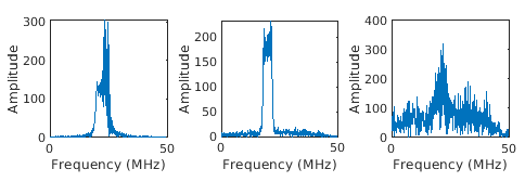
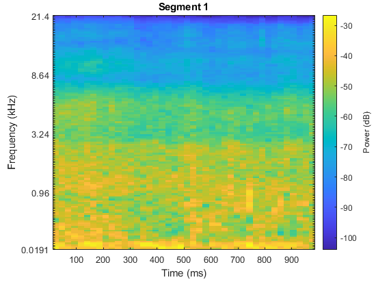
Synthetic pedestrian, car, and bicyclist backscattering
| Generate a synthetic pedestrian, car, and bicyclist
backscattering data set using the helper functions
The
helper function The helper function
To access these functions, open the example as a live script.
numPed = 1; % Number of pedestrian realizations
numBic = 1; % Number of bicyclist realizations
numCar = 1; % Number of car realizations
[xPedRec,xBicRec,xCarRec,Tsamp] = helperBackScatterSignals(numPed,numBic,numCar);

[SPed,T,F] = helperDopplerSignatures(xPedRec,Tsamp);
[SBic,~,~] = helperDopplerSignatures(xBicRec,Tsamp);
[SCar,~,~] = helperDopplerSignatures(xCarRec,Tsamp);
For an example showing how to process this data for deep learning, see Pedestrian and Bicyclist Classification Using Deep Learning (Radar Toolbox). | Sequence-to-label classification |
Generated waveforms
| Generate rectangular, linear FM, and phase coded waveforms
using the helper function
The
helper function To access these functions, open the example as a live script.
[wav, modType] = helperGenerateRadarWaveforms; For an example showing how to process this data for deep learning, see Radar and Communications Waveform Classification Using Deep Learning (Radar Toolbox). | Sequence-to-label classification |


Video Data Sets
| Data | Description | Task |
|---|---|---|
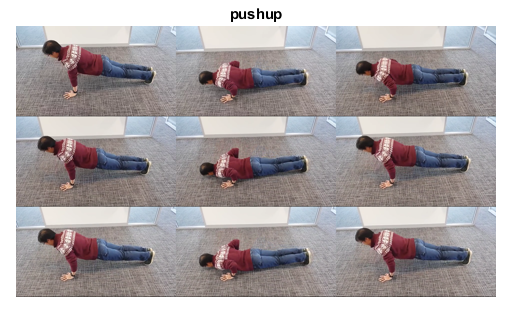
HMDB: a large human motion database
(Representative example) | The HMBD51 data set contains about 2 GB of video data for 7000 clips from 51 classes, such as drink, run, and pushup. Download and extract the HMBD51 data set from HMDB51: A Large Video Database for Human Motion Recognition. The data set is about 2 GB. After you extract the RAR files,
get the file names and the labels of the videos by using the helper
function dataFolder = fullfile(tempdir,"hmdb51_org");
[files,labels] = hmdb51Files(dataFolder);For an example showing how to process this data for deep learning, see Classify Videos Using Deep Learning. | Video classification |
Text Data Sets
| Data | Description | Task |
|---|---|---|
|
Factory Reports
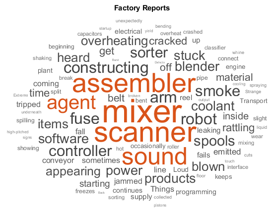
| The Factory Reports data set is a table containing approximately 500 reports with various
attributes including a plain text description in the variable Read the Factory Reports data from the file filename = "factoryReports.csv"; data = readtable(filename,'TextType','string'); textData = data.Description; labels = data.Category; For an example showing how to process this data for deep learning, see Classify Text Data Using Deep Learning. |
Text classification, topic modeling |
|
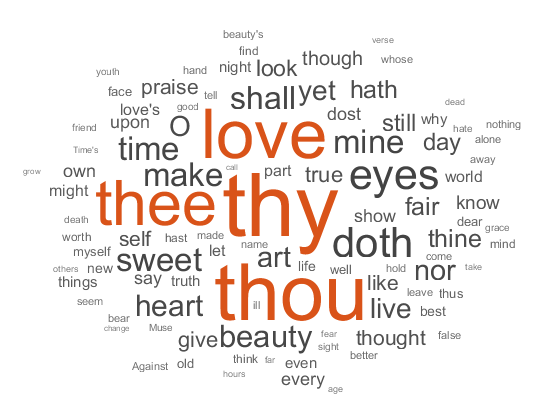
Shakespeare's Sonnets
| The file Read the Shakespeare's Sonnets data from the file
filename = "sonnets.txt";
textData = fileread(filename);
The sonnets are indented by two whitespace characters and are separated by two newline
characters. Remove the indentations using textData = replace(textData," ",""); textData = split(textData,[newline newline]); textData = textData(5:2:end); For an example showing how to process this data for deep learning, see Generate Text Using Deep Learning. |
Topic modeling, text generation |
|
ArXiv Metadata
| The ArXiv API allows you to access the metadata of scientific e-prints submitted to https://arxiv.org including the abstract and subject areas. For more information, see https://arxiv.org/help/api. Import a set of abstracts and category labels from math papers using the arXiV API. url = "https://export.arxiv.org/oai2?verb=ListRecords" + ... "&set=math" + ... "&metadataPrefix=arXiv"; options = weboptions('Timeout',160); code = webread(url,options); For an example showing how to parse the returned XML code and import more records, see Multilabel Text Classification Using Deep Learning. |
Text classification, topic modeling |
|
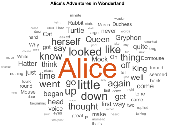
Books from Project Gutenberg
| You can download many books from Project Gutenberg. For example, download the text from Alice's Adventures in Wonderland by Lewis Carroll from https://www.gutenberg.org/files/11/11-h/11-h.htm using the url = "https://www.gutenberg.org/files/11/11-h/11-h.htm";
code = webread(url);The HTML code contains the relevant text inside tree = htmlTree(code);
selector = "p";
subtrees = findElement(tree,selector);Extract the text data from the HTML subtrees using the textData = extractHTMLText(subtrees);
textData(textData == "") = [];For an example showing how to process this data for deep learning, see Word-by-Word Text Generation Using Deep Learning. |
Topic modeling, text generation |
|
Weekend updates
| The file Extract the text data from the file filename = "weekendUpdates.xlsx"; tbl = readtable(filename,'TextType','string'); textData = tbl.TextData; For an example showing how to process this data, see Analyze Sentiment in Text (Text Analytics Toolbox). |
Sentiment analysis |
|
Roman Numerals
| The CSV file Load the decimal-Roman numeral pairs from the CSV file filename = fullfile("romanNumerals.csv"); options = detectImportOptions(filename, ... 'TextType','string', ... 'ReadVariableNames',false); options.VariableNames = ["Source" "Target"]; options.VariableTypes = ["string" "string"]; data = readtable(filename,options); For an example showing how to process this data for deep learning, see Sequence-to-Sequence Translation Using Attention. |
Sequence-to-sequence translation |
|
Finance Reports
|
The Securities and Exchange Commission (SEC) allows you to access financial reports via the Electronic Data Gathering, Analysis, and Retrieval (EDGAR) API. For more information, see https://www.sec.gov/search-filings/edgar-search-assistance/accessing-edgar-data. To download this data, use the function year = 2019; qtr = 4; maxLength = 2e6; textData = financeReports(year,qtr,maxLength); For an example showing how to process this data, see Generate Domain Specific Sentiment Lexicon (Text Analytics Toolbox). |
Sentiment analysis |


Audio Data Sets
| Data | Description | Task |
|---|---|---|
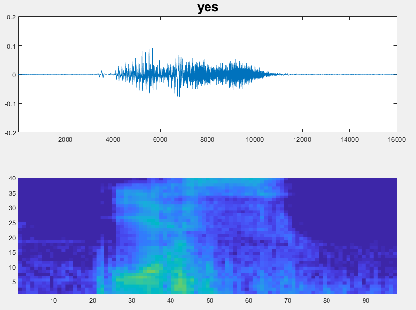
Speech Commands
| The Speech Commands data set consists of approximately 65,000 audio files labeled with 1 of 12 classes including yes, no, on, and off, as well as classes corresponding to unknown commands and background noise [35]. Download and extract the Speech Commands data set from https://storage.googleapis.com/download.tensorflow.org/data/speech_commands_v0.01.tar.gz. The data set is about 1.4 GB. Set
dataFolder = tempdir;
ads = audioDatastore(dataFolder, ...
    'IncludeSubfolders',true, ...
    'FileExtensions','.wav', ...
    'LabelSource','foldernames');
For an example showing how to process this data for deep learning, see Train Speech Command Recognition Model Using Deep Learning. | Audio classification, speech recognition |
Mozilla Common Voice
| The Mozilla Common Voice data set consists of audio recordings of speech and corresponding text files. The data also includes demographic metadata such as age and accent. Download
and extract the Mozilla Common Voice data set data set from https://commonvoice.mozilla.org/. The data set is
an open data set, which means that it can grow over time. As of
October 2019, the data set is about 28 GB. Set
dataFolder = tempdir;
ads = audioDatastore(fullfile(dataFolder,"clips")); | Audio classification, speech recognition. |
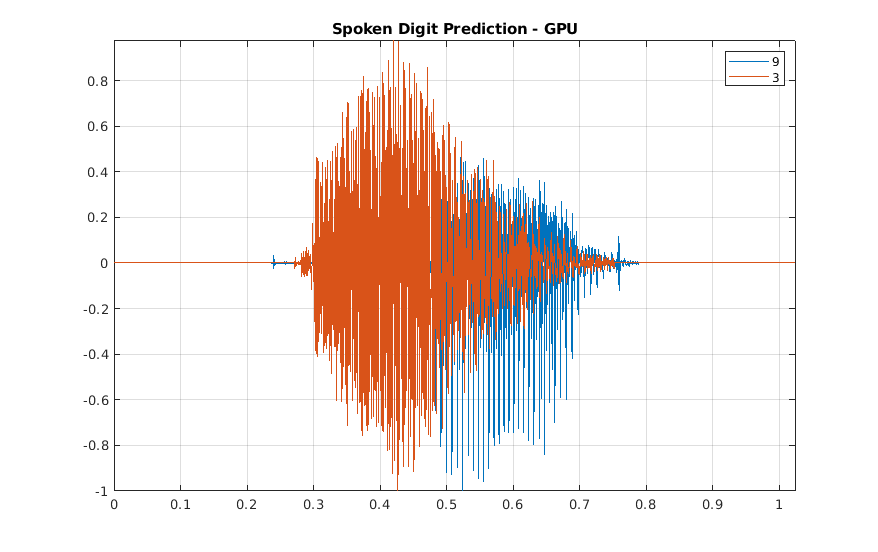
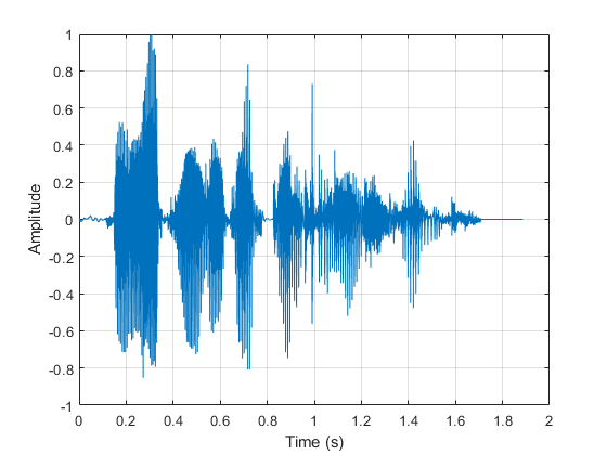
Free Spoken Digit Dataset
| The Free Spoken Digit Dataset, as of January 29, 2019, consists of 2000 recordings of the English digits 0 through 9 obtained from four speakers. Two of the speakers in this version are native speakers of American English and two speakers are nonnative speakers of English with a Belgium French and German accent respectively. The data is sampled at 8000 Hz. Download the Free Spoken Digit Dataset (FSDD) recordings from https://github.com/Jakobovski/free-spoken-digit-dataset. Set dataFolder = fullfile(tempdir,'free-spoken-digit-dataset','recordings'); ads = audioDatastore(dataFolder); For an example showing how to process this data for deep learning, see Spoken Digit Recognition with Wavelet Scattering and Deep Learning. | Audio classification, speech recognition. |
Berlin Database of Emotional Speech
| The Berlin Database of Emotional Speech contains 535 utterances spoken by 10 actors intended to convey one of the following emotions: anger, boredom, disgust, anxiety/fear, happiness, sadness, or neutral [36]. The emotions are text independent. The file names are codes indicating the speaker ID, text spoken, emotion, and version. The website contains a key for interpreting the code and additional information about the speakers such as age. Download the Berlin Database of Emotional Speech from http://emodb.bilderbar.info/index-1280.html. The data set is about 40 MB. Set dataFolder = tempdir;
ads = audioDatastore(fullfile(dataFolder,"wav"));
For an example showing how to process this data for deep learning, see Speech Emotion Recognition. | Audio classification, speech recognition. |
TUT Acoustic Scenes 2017
| The TUT Acoustic Scenes 2017 data set consists of 10-second audio segments from 15 acoustic scenes including bus, car, and library. Download and extract the TUT Acoustic Scenes 2017 data set from TUT Acoustic scenes 2017, Development dataset and TUT Acoustic scenes 2017, Evaluation dataset [37]. For an example showing how to process this data for deep learning, see Acoustic Scene Recognition Using Late Fusion. | Acoustic scene classification |
Point Cloud Data Sets
| Data | Description | Task |
|---|---|---|
WPI Lidar Data | The WPI Lidar data is collected using an Ouster OS1 sensor. It contains organized lidar point cloud scans of highway scenes and corresponding ground truth labels for car and truck objects. The data set has 1617 point clouds stored as Execute this code to download the data set. url = 'https://www.mathworks.com/supportfiles/lidar/data/WPI_LidarData.tar.gz'; outputFolder = fullfile(tempdir,'WPI'); lidarDataTarFile = fullfile(outputFolder,'WPI_LidarData.tar.gz'); if ~exist(lidarDataTarFile, 'file') mkdir(outputFolder); disp('Downloading WPI Lidar driving data (760 MB)...'); websave(lidarDataTarFile, url); untar(lidarDataTarFile,outputFolder); end lidarData = load(fullfile(outputFolder, 'WPI_LidarData.mat')); WPI_LidarData folder. If you do so, change
the outputFolder variable in the code to the
location of the downloaded file.For an example showing how to process this data for deep learning, see Lidar Point Cloud Semantic Segmentation Using PointSeg Deep Learning Network. | Semantic segmentation |
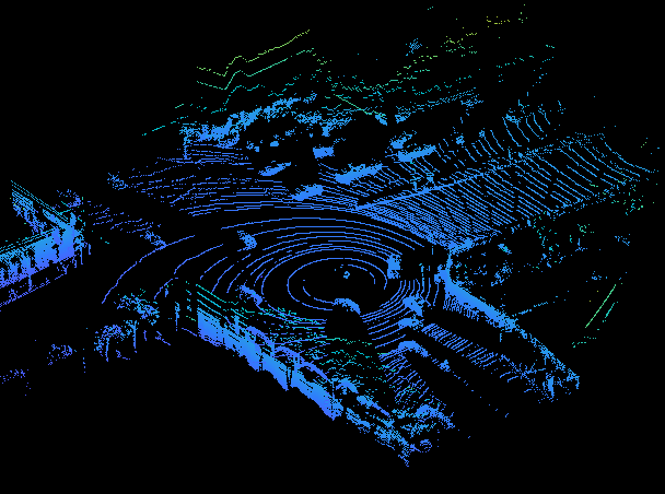
PandaSet Data | PandaSet contains 2560 organized lidar point cloud scans of various city scenes captured using the Pandar 64 sensor. The data set provides semantic segmentation labels for 12 different classes and 3-D bounding box information for three classes, which are car, truck, and pedestrian. The size of the data set is 5.2 GB. Execute this code to download the data set. url = 'https://ssd.mathworks.com/supportfiles/lidar/data/Pandaset_LidarData.tar.gz'; outputFolder = fullfile(tempdir,'Pandaset'); lidarDataTarFile = fullfile(outputFolder,'Pandaset_LidarData.tar.gz'); if ~exist(lidarDataTarFile, 'file') mkdir(outputFolder); disp('Downloading Pandaset Lidar driving data (5.2 GB)...'); websave(lidarDataTarFile, url); untar(lidarDataTarFile,outputFolder); end lidarData = fullfile(outputFolder,'Lidar'); labelsFolder = fullfile(outputFolder,'semanticLabels'); Depending
on your internet connection, the download process can take some
time. Alternatively, you can download the data set to your local
disk from your web browser using the URL, and then extract the
For examples showing how to process this data for deep learning, see Lidar Point Cloud Semantic Segmentation Using SqueezeSegV2 Deep Learning Network and Lidar 3-D Object Detection Using PointPillars Deep Learning. | Object detection, Semantic segmentation |

References
[1] Lake, Brenden M., Ruslan Salakhutdinov, and Joshua B. Tenenbaum. “Human-Level Concept Learning through Probabilistic Program Induction.” Science 350, no. 6266 (December 11, 2015): 1332–38. https://doi.org/10.1126/science.aab3050.
[2] The TensorFlow Team. "Flowers" https://www.tensorflow.org/datasets/catalog/tf_flowers.
[3] Kat, Tulips, image, https://www.flickr.com/photos/swimparallel/3455026124. Creative Commons License (CC BY).
[4] Rob Bertholf, Sunflowers, image, https://www.flickr.com/photos/robbertholf/20777358950. Creative Commons 2.0 Generic License.
[5] Parvin, Roses, image, https://www.flickr.com/photos/55948751@N00. Creative Commons 2.0 Generic License.
[6] John Haslam, Dandelions, image, https://www.flickr.com/photos/foxypar4/645330051. Creative Commons 2.0 Generic License.
[7] Krizhevsky, Alex. "Learning Multiple Layers of Features from Tiny Images." MSc thesis, University of Toronto, 2009. https://www.cs.toronto.edu/%7Ekriz/learning-features-2009-TR.pdf.
[8] Brostow, Gabriel J., Julien Fauqueur, and Roberto Cipolla. “Semantic Object Classes in Video: A High-Definition Ground Truth Database.” Pattern Recognition Letters 30, no. 2 (January 2009): 88–97. https://doi.org/10.1016/j.patrec.2008.04.005.
[9] Kemker, Ronald, Carl Salvaggio, and Christopher Kanan. “High-Resolution Multispectral Dataset for Semantic Segmentation.” ArXiv:1703.01918 [Cs], March 6, 2017. https://arxiv.org/abs/1703.01918.
[10] Isensee, Fabian, Philipp Kickingereder, Wolfgang Wick, Martin Bendszus, and Klaus H. Maier-Hein. “Brain Tumor Segmentation and Radiomics Survival Prediction: Contribution to the BRATS 2017 Challenge.” In Brainlesion: Glioma, Multiple Sclerosis, Stroke and Traumatic Brain Injuries, edited by Alessandro Crimi, Spyridon Bakas, Hugo Kuijf, Bjoern Menze, and Mauricio Reyes, 10670: 287–97. Cham, Switzerland: Springer International Publishing, 2018. https://doi.org/10.1007/978-3-319-75238-9_25.
[11] Ehteshami Bejnordi, Babak, Mitko Veta, Paul Johannes van Diest, Bram van Ginneken, Nico Karssemeijer, Geert Litjens, Jeroen A. W. M. van der Laak, et al. “Diagnostic Assessment of Deep Learning Algorithms for Detection of Lymph Node Metastases in Women With Breast Cancer.” JAMA 318, no. 22 (December 12, 2017): 2199. https://doi.org/10.1001/jama.2017.14585.
[12] McCollough, C.H., Chen, B., Holmes, D., III, Duan, X., Yu, Z., Yu, L., Leng, S., Fletcher, J. (2020). Data from Low Dose CT Image and Projection Data [Data set]. The Cancer Imaging Archive. https://doi.org/10.7937/9npb-2637.
[13] Grants EB017095 and EB017185 (Cynthia McCollough, PI) from the National Institute of Biomedical Imaging and Bioengineering.
[14] Grubinger, Michael, Paul Clough, Henning Müller, and Thomas Deselaers. "The IAPR TC-12 Benchmark: A New Evaluation Resource for Visual Information Systems." Proceedings of the OntoImage 2006 Language Resources For Content-Based Image Retrieval. Genoa, Italy. Vol. 5, May 2006, p. 10.
[15] Ignatov, Andrey, Luc Van Gool, and Radu Timofte. “Replacing Mobile Camera ISP with a Single Deep Learning Model.” ArXiv:2002.05509 [Cs, Eess], February 13, 2020. https://arxiv.org/abs/2002.05509. Project Website.
[16] Chen, Chen, Qifeng Chen, Jia Xu, and Vladlen Koltun. “Learning to See in the Dark.” ArXiv:1805.01934 [Cs], May 4, 2018. https://arxiv.org/abs/1805.01934.
[17] LIVE: Laboratory for Image and Video Engineering. https://live.ece.utexas.edu/research/ChallengeDB/index.html.
[18] Özgenel, Ç. F., and Arzu Gönenç Sorguç. “Performance Comparison of Pretrained Convolutional Neural Networks on Crack Detection in Buildings.” Taipei, Taiwan, 2018. https://doi.org/10.22260/ISARC2018/0094.
[19] Zhang, Lei, Fan Yang, Yimin Daniel Zhang, and Ying Julie Zhu. “Road Crack Detection Using Deep Convolutional Neural Network.” In 2016 IEEE International Conference on Image Processing (ICIP), 3708–12. Phoenix, AZ, USA: IEEE, 2016. https://doi.org/10.1109/ICIP.2016.7533052.
[20] Wu, Ming-Ju, Jyh-Shing R. Jang, and Jui-Long Chen. “Wafer Map Failure Pattern Recognition and Similarity Ranking for Large-Scale Data Sets.” IEEE Transactions on Semiconductor Manufacturing 28, no. 1 (February 2015): 1–12. https://doi.org/10.1109/TSM.2014.2364237.
[21] Jang, Roger. "MIR Corpora." http://mirlab.org/dataset/public/.
[22] Huang, Weibo, and Peng Wei. "A PCB dataset for defects detection and classification." arXiv preprint arXiv:1901.08204 (2019). https://arxiv.org/abs/1901.08204.
[23] Synthetic PCB Dataset. https://github.com/Ironbrotherstyle/PCB-DATASET.
[24] Zou, Yang, Jongheon Jeong, Latha Pemula, Dongqing Zhang, and Onkar Dabeer. "SPot-the-Difference Self-supervised Pre-training for Anomaly Detection and Segmentation." In Computer Vision–ECCV 2022: 17th European Conference, Tel Aviv, Israel, October 23–27, 2022, Proceedings, Part XXX, pp. 392-408. Cham: Springer Nature Switzerland, 2022. https://arxiv.org/pdf/2207.14315v1.
[25] Visual Anomaly (VisA) Dataset. https://github.com/amazon-science/spot-diff/tree/main.
[26] Al-Dhabyani, Walid, Mohammed Gomaa, Hussien Khaled, and Aly Fahmy. “Dataset of Breast Ultrasound Images.” Data in Brief 28 (February 2020): 104863. https://doi.org/10.1016/j.dib.2019.104863.
[27] Frazier, J. A., S. M. Hodge, J. L. Breeze, A. J. Giuliano, J. E. Terry, C. M. Moore, D. N. Kennedy, et al. “Diagnostic and Sex Effects on Limbic Volumes in Early-Onset Bipolar Disorder and Schizophrenia.” Schizophrenia Bulletin 34, no. 1 (October 27, 2007): 37–46. https://doi.org/10.1093/schbul/sbm120.
[28] Radau, Perry, Yingli Lu, Kim Connelly, Gideon Paul, Alexander J Dick, and Graham A Wright. “Evaluation Framework for Algorithms Segmenting Short Axis Cardiac MRI.” The MIDAS Journal, July 9, 2009. https://doi.org/10.54294/g80ruo.
[29] Kudo, Mineichi, Jun Toyama, and Masaru Shimbo. "Multidimensional Curve Classification Using Passing-through Regions." Pattern Recognition Letters 20, no. 11–13 (November 1999): 1103–11. https://doi.org/10.1016/S0167-8655(99)00077-X.
[30] Kudo, Mineichi, Jun Toyama, and Masaru Shimbo. Japanese Vowels Data Set. Distributed by UCI Machine Learning Repository. https://archive.ics.uci.edu/ml/datasets/Japanese+Vowels
[31] Saxena, Abhinav, Kai Goebel, Don Simon, and Neil Eklund. "Damage propagation modeling for aircraft engine run-to-failure simulation." In Prognostics and Health Management, 2008. PHM 2008. International Conference on, pp. 1-9. IEEE, 2008.
[32] Rieth, Cory A., Ben D. Amsel, Randy Tran, and Maia B. Cook. "Additional Tennessee Eastman Process Simulation Data for Anomaly Detection Evaluation." Harvard Dataverse, Version 1, 2017. https://doi.org/10.7910/DVN/6C3JR1.
[33] Goldberger, Ary L., Luis A. N. Amaral, Leon Glass, Jeffrey M. Hausdorff, Plamen Ch. Ivanov, Roger G. Mark, Joseph E. Mietus, George B. Moody, Chung-Kang Peng, and H. Eugene Stanley. "PhysioBank, PhysioToolkit, and PhysioNet: Components of a New Research Resource for Complex Physiologic Signals." Circulation 101, No. 23, 2000, pp. e215–e220. https://www.ahajournals.org/doi/full/10.1161/01.cir.101.23.e215.
[34] Laguna, Pablo, Roger G. Mark, Ary L. Goldberger, and George B. Moody. "A Database for Evaluation of Algorithms for Measurement of QT and Other Waveform Intervals in the ECG." Computers in Cardiology 24, 1997, pp. 673–676.
[35] Warden, Pete. "Speech Commands: A public dataset for single-word speech recognition", 2017. Available from http://download.tensorflow.org/data/speech_commands_v0.01.tar.gz. Copyright Google 2017. The Speech Commands Dataset is licensed under the Creative Commons Attribution 4.0 license, available here: https://creativecommons.org/licenses/by/4.0/legalcode.
[36] Burkhardt, Felix, Astrid Paeschke, Melissa A. Rolfes, Walter F. Sendlmeier, and Benjamin Weiss. "A Database of German Emotional Speech." Proceedings of Interspeech 2005. Lisbon, Portugal: International Speech Communication Association, 2005.
[37] Mesaros, Annamaria, Toni Heittola, and Tuomas Virtanen. "Acoustic scene classification: an overview of DCASE 2017 challenge entries." In 2018 16th International Workshop on Acoustic Signal Enhancement (IWAENC), pp. 411-415. IEEE, 2018.
[38] Hesai and Scale. PandaSet. https://pandaset.org/
See Also
trainnet | trainingOptions | dlnetwork