Mixed-Signal Analyzer part 2: Automation
From the series: Mixed-Signal Data Analysis with MATLAB
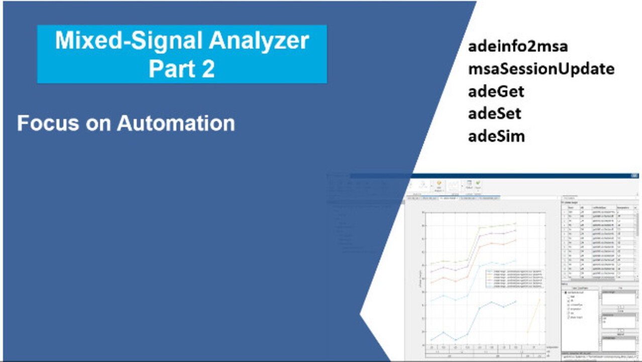
This continuation video on Mixed-Signal Analyzer picks up where our introductory video left off. The focus in this video is on automation. We start by saving our Cadence simulation data to .mat files using the adeinfo2msa function. This allows us to post-process our data on either Linux or Windows. In our case, we used Windows. Next, we show how to apply a past Mixed-Signal Analyzer session to new simulation data. This macro-like capability allows you to automate past analyses on new data without any point and click. Finally, we introduce additional automation functionality by way of adeGet, adeSet, and adeSim. These functions allow for an automated round-trip workflow between Virtuoso and MATLAB.
Published: 11 Feb 2024
Hello this is Kerry Schutz with MathWorks, and this is Part 2 in my series on using Mixed-Signal Analyzer for analyzing Cadence simulation data. In the previous video, I did a number of things. I walked through the Cadence project, which was a low-dropout regulator.
And I just showed a series of steps from that point forward. I showed how you could move from the Cadence environment to the MATLAB environment and create an adeInfo object using the M-button in Cadence. We open Mixed-Signal Analyzer. And then we imported the data using that adeInfo object. It's a MATLAB variable which points to your Cadence data.
Then I displayed a number of things. I looked at the LDO-out signal, DC analysis, transient analysis. I looked at a number of metrics. And I plotted those metrics as trend charts. I did about three of those trend charts. And then before that, some of those trend charts were the result of custom analyses I did on certain waveforms.
Finally, to avoid having to reproduce that setup each time I want to look at the data, I save that LDO session to a session file, which is a .mat file. I generated a PDF report, and I did all of that work on Linux, the same environment where I was running the Cadence tools.
In this video, I'm going to pick up where we left off here. Now, instead of working with the adeInfo object, I'm going to convert the data, save it to a mat file first on the Linux environment. And then I'm going to copy those mat files over to the Windows environment and work with Mixed-Signal Analyzer, the app, on Windows.
I'm going to open that LDO session that we saved in our first video. And then we'll look, make sure the data is all looking the same as if it were on the Cadence side-- just a quick sanity check. And then we'll update that session with another set of data. So we'll take another interactive run in Cadence. We'll point to that instead. And then we'll apply the same sorts of visualizations and analysis as we did before.
We're going to look and see how the phase margin information is different between the two. Remember, I changed some parameters when going from one interactive run to the next. And I'll show that again. And then I'm going to look at a couple interactive commands that allow you to control or interact with Cadence from the MATLAB side. There's three of those, adeGet, adeSet, and adeSim, which kind of work the way you would think for getting variables, setting variables, and for simulating with these three commands.
OK. So let's jump right into the steps. OK. Now we're over in MATLAB under Linux and R2023b. And if you recall from our previous video, we had saved our data to LDO_SESSION.mat. That was all the plots, visualizations, trend charts that we had done inside of Mixed-Signal Analyzer. Now, what I want to do now is take our adeInfo object, or the data pointed to by it, over in Cadence and save it to a mat file.
So in order to do that, I'm going to take advantage of a command called adeInfo2ms-a. I'm going to up arrow since I've already called this command in the past. And I'm going to say, I want to save Interactive run 190. I don't want to open up Mixed-Signal Analyzer. So that's why this is set to false-- import2msa, false.
And I don't just want the metrics only. I want the waveforms as well. So that's going to be set to false as well. Now, there's a number of other parameters you can also set. With this particular function, I'm just going to use these three right now. So I'll execute that command. It's going to extract the simulation data. We'll just let that complete, and it's done. And it says a few things. One is it created this ldo_test_Interactive.190.mat file that you see here. Also created ldo_test-Interactive.190 folder, which contains waveform data. And that's right here. So if we expand that, we'll see it it's got a couple files inside of that.
All right. So we've got essentially two things created, a file here and a folder here. The file here contains metrics data. The folder here contains waveform data. And now we could go off into Mixed-Signal Analyzer and work with the file instead of the adeInfo object. We could also save other runs to a file. I'm going to do 191 as well-- same thing, everything else the same. Run that. And we're done, and now you can see we've got the 190 and the 191 folder as well.
All right. So let's go ahead and open up Mixed-Signal Analyzer and work with-- oh, well, before we do that, we're not going to, this time, work with the data on Linux side. We're going to copy this data over to Windows and work with this data on the Windows side. OK. So voila. Now I'm under MATLAB-- same version under Windows now. You see the two mat files and the two folders that were created, again, holding waveform data, holding metrics data-- and also our session file as well. So let's open up Mixed-Signal Analyzer on Windows-- same process. Just type "mixedsignalanalyzer," or go to the Apps tab.
OK. The first thing let's do is just do a quick sanity check to make sure that we can look at the data on both sides. So I've copied not just the data files. I also copied the session file over so we can open that up. And now let's see if we can-- basically make sure we can do the same analysis visualizations here on Windows.
And it's almost done here. We're on our fifth plot, and we could quickly go through these. Here's the slewrate plot, the max of LDO out, the phase margin, the TRAN of LDO out, and the DC waveform LDO out. All right. And if we just do a quick study of the phase margin plot, we're going to see we've got plots that go anywhere from down here around 48 to 54. This one starts around 54, goes up to about 60. Some of these start around 60, go up to anywhere from 62 to 66 degrees in phase margin. OK. So just to keep a quick sanity check on that-- about 48 up to about 66 as far as the phase margin data for that particular Interactive 190 run.
Now what we want to do is do the same analysis, same visualizations on Interactive run 190. So how can we do that? One is you could say, well, I want to update this session with another file. And I'm going to say, select the 191 Interactive run. Say Open. And I'll let it go. And it'll start doing the update process. I need to say, OK, we're going to replace 190 with 191. Say Refresh. And it'll start the update process. We'll let that go to finish.
OK. So we finished the update process, and we've got the same visualization, same TRAN charts up. Notice it does say "191" over here, not "190" anymore. Let's go to the phase margin plot and look at the range of values. The plots go from about 58 up to about 74, 75 for the phase margin in degrees. So we can see we definitely have an improved phase margin overall using the different values in that simulation, which happen to be different CFB, or different feedback capacitor values, which in this case were 30 and 35 femto as different from the Interactive 190, which was 20 and 25 femto.
Now as before, of course we could go off and export a generated report. We won't do that again here. Another thing we can do is everything I just did point and click to do the update, we could also do that programmatically. So let's go off and do that.
What I'm going to do to demonstrate that capability is we're now going to update the 190-- well, we could if we had 192, or another one we could do that. In this case, I'm just going to go back to 190 where we started. But I'm going to do that. I'm going to update the data with the 190. Again, I could go here and select the 190 data. I could say, Update, select the 190 data where I started, or cancel that out. What I'm going to do is do that programmatically.
So we'll go over to the MATLAB environment to do that. We're going to take advantage of another command, and instead of adeInfo2ms-a, that function, we are going to use msaSessionUpdate. We're going to specify the name of the session file that we're using, which is what we have open now, the old session. And we're going to update that with 190 interactive run 190, where, again, we're sitting right now at 191. So let's go ahead and execute that command. And that'll go off and run.
OK. After finishing that update, you can now see that we've got interactive 190 in here again. And you can see definitely the phase margin is back to the lower phase margins, from about 48 up to about 66, depending on which particular simulation case we are running.
So again, there are two ways to do the update when you have a new data set. You could go to the update menu and select the file that you want to update with. Or you could go to the MATLAB prompt or your script and execute the MSA session update function, telling it which kind of analysis you want to apply from the session file and what the new data file is that's going to be analyzed.
OK. So next, let's look at some of the interactive commands, adeGet, adeSet, and adeSim. Now first, in order to leverage those three interactive commands, adeGet, adeSet, and adeSim, I'm going to have to go back to the Linux side, back to the Linux session of MATLAB, where the adeInfo object existed. Notice, I don't have an adeInfo object on my Windows side because that's not where my Cadence environment is running. I'm not connected to Virtuoso on the windows side.
So let me go back to my session on the Linux side. All right. Now, here we are over on the Linux side in MATLAB 23b. And here I have my adeInfo object. And now I'm going to type a-d-e lowercase and capital G-e-t. And it's going to tell me what kind of variables I have access to here, like vdd, Iload, cfb, et cetera. OK?
Now, that's not telling me their values. That's just telling me what I have access to. If I want to get one of their values, I could elaborate on the adeGET command, and I could say something like, "varName" is equal to, let's say, cfb, the capacitor. And let's just get those values. And it tells me, they are currently set to 20 and 25 femtofarads. And you could see that over here in my Virtuoso Maestro setup.
Now, if I wanted to change them, I could use the adeSet command. And I'll do that, adeSet, varName cfb. And we'll say varValue equal to-- in single parentheses, we could put 40f and 45f, let's say. And now keep your eye on cfb over here. And we've changed it. OK, great. And if we don't want to keep it, we could always just change it back to what we had.
And you'll see it change over here. Excellent. Now finally, if I wanted to rerun the simulation with whatever new variables I had set from the MATLAB side without going over to Virtuoso, I could just type adeSim, and it will use whatever my current settings are, current variable names are, and create a new interactive run from which we can, again, grab the data and update my session in Mixed-signal Analyzer and continue that back and forth interactive workflow.
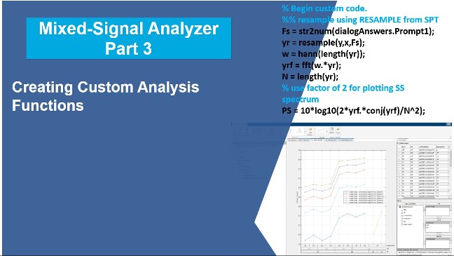
All right. That's all I'm going to cover in this video on Mixed-Signal Analyzer. In the follow-on video, I'll cover a few more features, like custom functions Thank you.


Seleccione un país/idioma
Seleccione un país/idioma para obtener contenido traducido, si está disponible, y ver eventos y ofertas de productos y servicios locales. Según su ubicación geográfica, recomendamos que seleccione: United States.
También puede seleccionar uno de estos países/idiomas:
América
- América Latina (Español)
- Canada (English)
- United States (English)
Europa
- Belgium (English)
- Denmark (English)
- Deutschland (Deutsch)
- España (Español)
- Finland (English)
- France (Français)
- Ireland (English)
- Italia (Italiano)
- Luxembourg (English)
- Netherlands (English)
- Norway (English)
- Österreich (Deutsch)
- Portugal (English)
- Sweden (English)
- Switzerland
- United Kingdom (English)