Mixed-Signal Analyzer part 3: Custom analysis functions

Hello, this is Kerry Schutz with MathWorks. And this is part 3 in our series of videos on using Mixed-Signal Analyzer to post-process and analyze cadence simulation data. In this video, we're going to concentrate on how to create and apply custom analysis functions. Our design in this case is going to be a clock buffer design. There are multiple stages. And we're going to be varying certain parameters, certain passive values, and certain transistor parameters, transistor widths, et cetera.

This is our setup in Maestro. Again, we've conducted different types of analyses, tran and dc. There are different design variables. We've got different corner setups. And we've computed different metrics. We've done a number of interactive runs. And finally, we're to the point where we're going to click on the end button, the MATLAB button, to create this adeInfo object in MATLAB. And that will be able to access our simulation results with on the MATLAB side.

Here's our adeInfo object in MATLAB. Again, it's a pointer to the data, not the data itself. If we want the data itself, we want to save it to a MAT file, we're going to leverage the adeinfo2msa function, part of Mixed-Signal block set. And there are a number of parameters you can specify, like do you want the metrics only or do you want the waveform data? And then, of course, which interactive run do you want to save?

So, we've done that in this case already. And we have also taken that resulting MAT file and copied it over from the Linux side over to a Windows machine. And we're going to do the post-processing using Mixed-Signal Analyzer from Windows. And finally, this is where we're going to start the thrust of today's video. We're going to open up Mixed-Signal Analyzer in Windows. We're going to say, Import File, and open up those MAT files.

OK, so, here we are over in MATLAB R2023b in Windows. We've got our clockBuffer.mat file. And then, we've got our clock buffer folder with our waveform data. I'm going to open up Mixed-Signal Analyzer. All right, now, with Mixed-Signal Analyzer open, we're ready to import our data. So, I'll go to Import File, point to our clockBuffer.mat file. That's going to load in.

You can see here, the name of our run. It was Interactive Run 2 bash test, was the name of the test, and 80 cases, one point sweep, 80 corners. And then, you see our transient signals we logged, our dc signals, dc analysis. And then, we computed a number of metrics. So, if we wanted to look at, let's say, tran01, that would be as simple as selecting tran01 and saying, display waveform. That's going to display the signal and the time domain of all ad corners.

Now, of course, we could always simplify that and say, well, I don't want all ad corners. I just want one, and let's say 10, and maybe six, something like that. Or you could go back and display them all. All right, we did all of that in our previous videos, how to do filtering and applying different analysis to the data. Now, in this video, what we want to do is assume that there wasn't necessarily a function built into Mixed-Signal Analyzer that you could use. So, you had to write your own.

Now, in this case, I'm going to select 01 again. I'm going to add a new plot. And I had already created a new analysis called MySpectrum. Now, it just so happens, in this case, there is a power spectrum function built into Mixed-Signal Analyzer. But it could be that either, a, that function didn't exist. So, you'd have to create one. Or maybe you just want to do a custom version of the power spectrum calculation. So, you still want to write your own or leverage your own existing scripts or functions.

So, here, I've created my own. So, if I wanted to select and apply this analysis to this signal or this waveform, you just select it. Click MySpectrum. And in this case, it's asking for a couple of additional input parameters. I'm going to say the sample rate for my analysis is 40 gigahertz. And I'm going to display it in log format. Now, the reason these prompts are there, well, obviously, it's for some level of customization.

But the sample rate is there in particular because, if you recall, the data in general from spectra or from a SPICE simulator is variable step. And when you're going to do frequency domain or spectral analysis, typically, you want to have a fixed step or a fixed sample rate on that data to apply the FFT. So, in this case, I'm using 40 gigahertz. And we're going to display it using log x-axis.

All right, so, that doesn't display anything immediately. But it does put the analysis under analysis waveforms. Now, if you select it and hit Display Waveform, you are going to get the spectrum across all 80 corners. So, I did, essentially, 80 FFTs and windowing, et cetera, and displayed the result right here on plot 2. Of course, as I've shown in previous videos, we could go in and customize these names. I'm not going to repeat all those steps here.

All right, so, if we wanted to know where that peak was, it looks like the first harmonic or the main frequency here of this clock is around 630 or so megahertz. OK, of course, there are also all the harmonics, the integer multiples of that 630 some odd megahertz signal. All right, so, next, we want to know, well, how can you create a function like this on your own? All right, so, the first thing you do anytime you want to analyze a signal is, you select the signal you want to analyze.

And so, I'm going to go under tran. I analyzed 01 before the spectrum using the one I already had in my custom analysis. So, I'm going to select 02 just to be different this time. And I'm going to say, Add Analysis. That that'll call up a dialogue where you can either enter a MATLAB expression. Remember, we did that in an earlier video. We entered something to compute the mean or the absolute value of the slew rate.

But again, sometimes, you need something more involved than a MATLAB one-liner. And you may need to pass parameters. And so, that's what a MATLAB function buys you. And now, we're going to enter the name of our new function. And this can be something, again, you haven't necessarily written yet. This is going to create a template for us. And I'll just call this MySpectrum2, to distinguish it from the previous one, MySpectrum.

And I'm going to have two prompts in this case. If you recall, before, I had sample rate and then the x-axis scaling. I'll do the same thing here. I'll say sample rate. And I'll say, we're going to specify in hertz. And I'll put a colon. And then, for the prompt two, I hit Enter. And I'll say x-axis scaling. And I'll put some kind of something. Hint to the user, I'll say linear equals 0 or log equal 1, colon.

So, they'll either enter a 0 or a 1, say, OK. That is going to give us a template with our new function, MySpectrum2. It's going to have two inputs, actually three inputs. The x is the time data. Y is the voltage. It's the amplitude data. And then, the prompt will be in the form of dialogue answers. And then, we'll have our outputs. Notably, the x-axis, in this case, it's going to be our frequency vector. And y-out is going to be our, let's say, watts or dbwatts, something like that.

All right, so, let's go down here. There are some things, hints that tells you what things are. I just mentioned x1 and x and y and dialogue answers. The outs, I mentioned. And then, there are these things called name value pairs, which give you some kind of customization options. Is the x units going to be time or is it going to be frequency? Is the x scale going to be linear or log? And what kind of x and y labels do you want?

OK, so, let's go down here, where the first section of code is on the arguments. And these are the prompts. Remember, we had two prompts, one for the sample rate and one for the x-axis scaling, linear or log. Now, we don't need to modify this section of code. But we do need to take actions based on what the user specified for linear and log here. Now, do note that the default prompt 1 is just a string of 0. And the default for prompt 2, which is a scaling, is also a string, just a 0.

Now, of course, the sample rate is going to be some number. It's not going to be zero and our scaling. Well, it could be zero. Or it could be 1. First thing I'm going to do is, under Initialize Return Values, is, I'm going to paste in some code here. And I'll explain what I'm doing here in a moment. I'm going to paste that in. And what I'm doing is, I'm overriding name value pairs. So, I'm going to get rid of this one. This line doesn't serve any purpose anymore, OK?

So, before, I just had this, and then that empty cell array for name value pairs. I'm going to replace it with, if, dialogue prompt 2, which is the x-axis scaling, is 1, that means log. Then, I'm going to set the x scale element of name value pairs to log. I'm always going to use-- my x scaling is going to be megahertz. I just know that's how my date is scaled best. And I'm always going to have my y label in terms of dB watts. That's just what I'm going to do.

I haven't shown the computations yet. And, of course, I'm plotting power spectrum. So, the x is going to be frequency. Now, if it happens to be linear, that's going to be if the prompt is not a 1. It's going to be a 1 or a 0. So, I just say, else, the x scale is going to be linear. And everything else is the same as before. Now, of course, I'm not being super careful here. In case, the user typed in 2, it would still go to this line right here. So, I'm not being that careful.

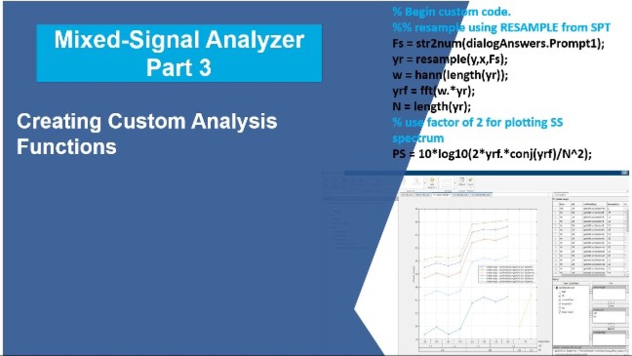
Now, we got a next section where we actually begin our custom code. And that's where we're going to compute our spectrum. Now, for this, you probably wanted to do some, or maybe you had an existing script which computed the spectrum. So, I'm going to go over to a script which I've already created for computing the spectrum, my spectrum post-processing script, or processing script.

And what I do here is I say, well, I've got a waveform with time values. And why, in fact, I'll just put that in there. I'll say, figure plot t1, comma, y1 and grid on, OK? And I won't bother with the x-axis labels. So, we'll just run maybe these lines of code right here. Let's just run that right there. And when we do that, we'll see our waveform that we're going to compute the spectrum of-- OK, so, square width.

Now, I'm going to skip a lot of the details here. But basically, we're just assuming we've got some data. And this is our practice script. We want to make sure our spectrum computation is working before we actually make it part of the MSA app. I'm going to choose a sample rate of 40 gigahertz, 40 gig samples per second. And then, I'm going to do some re-sampling. And the reason I'm doing the re-sampling is because my data that is in my original data set is not equally-sampled spaced in time. It's not a fixed sample rate.

And I've got a few lines of code here which kind of demonstrate that. I could uncomment this. I could take this section of code. If you actually want to see what the sample rate is, I could just execute these lines of code. And what you'll see is that the sample rate changes with time, OK? And from that, I said, OK, I'm going to pick a sample rate that's most appropriate.

It's not based on necessarily the peak. It's not based on the mean. There's some kind of scheme I had or you could use to pick the sample rate. One of them might be the median of those numbers. But you probably want to histogram it. And then, choose the sample rate again very carefully based on the spread and the sample times.

OK, so, I chose 40 gigahertz. I re-sample my data at that rate. So, I submit the original points, x and y or t and y1. And then, new sample rate, I get the new sample waveform. And then, what I do now is I start doing my spectral process. First thing I do is, I apply a hand window. I compute the FFT of that result. Or actually, I apply the window and take the FFT of that product.

And then, I compute the power spectrum, which is nothing more than the FFT, in this case, windowed, windowed times its complex conjugate divided by the number of points squared, 10 log 10 thereof. And then, because I'm using a single-sided spectrum, there's a factor of 2 in there. I have to double up on the energy to keep the energy preserved. Yeah, and then, what I do is, then, I just pull off the first half of the signal.

So, I'm not looking at the negative frequencies. I'm only looking at the data from 0 to Fs over 2, or 0 to 20 gigahertz, in this case. And then, I form my frequency vector based on that 20 gigahertz, our Fs over 2 value. And then, I divide it by 1e6 because I'm going to display the units, remember, in megahertz.

If you recall, in my script, MySpectrum2, I set the x label to be megahertz. So, I have to have the numbers scale in the x-axis accordingly. And we can run this. And we're going to see our spectrum. And again, this is just in MATLAB with our sample data set where we're just testing out our script before we make it and build it into Mixed-Signal Analyzer.

OK, so, that's good. So, now, we want to take this work. We want to take what we did here from about this point, down, and build this into our app. So, I'm going to copy this section of code, let's say down to here. I don't need-- when you're going to bring something into Mixed-Signal Analyzer or custom function, you don't need the actual plotting commands because that's handled separately from the custom analysis script.

So, I'm just going to copy that. OK, so, with that copied, we're going to go over to our MySpectrum2 function, our new one. And we're going to paste that into the Begin Custom Code section, OK? So, now, we come in. Now, we can't leave the Fs equals 49 here because this is a parameter which is one of the inputs. So, it could be anything.

So, Fs, in this case, is going to be equal to string to num of prompt 1. So, I'm going to copy that one. I'm going to paste it here. I'm going to change it to prompt 1, since that was what the user specified. Remember, it's input as a string. And then, you convert it to a number. And then, the rest of it just flows. And we compute, in this case, PS and fvec.

However, computing PS and fvec is not quite sufficient because if you recall, our output variables are Xout and Yout. So, we have to assign those appropriately. So, x out is going to be equal to fvec. And Yout is going to be equal to PS. And with that we should be good. So, I'm going to save that. And OK, so, let's give that a shot back in Mixed-Signal Analyzer.

Now, I should mention before I go to Mixed-Signal Analyzer where this file resides. When it created this new MySpectrum2 function, it's under your appdata roaming MathWorks MATLAB version number Plus, it is a custom folder that saved in this directory. Then, the next logical question is, why did it save or create this new custom analysis function in this very long path, this custom folder?

The reason is, it's because the app can always find your custom analysis function. There, it doesn't have to go searching around the entire MATLAB path to find them. They're in one central location. And this is the spot where it always looks for Mixed-Signal Analyzer custom analysis functions, which is essentially called your prefdir with the extra customization for MSA, which is the MS blocks plus MSA custom.

OK, again, I mentioned prefdir. That is a special directory that MATLAB applications always know about. You can type prefdir. And it'll tell you C: Users. K shoots out to R 2023b. And then, again, like I said, we added on the extra two extensions. We can go to those extensions. We'll find the MySpectrum function there and then the new one I created, MySpectrum2.

All right, so, now, let's go try to use that. We'll go back to Mixed-Signal Analyzer. Always select your signal of interest first if you want to analyze. Go to MySpectrum or MySpectrum2. I'll select it. It should prompt us with two prompts. For the sampler, I'll select 50 gigahertz this time. And I'll use linear scaling that's a 0. Hit OK. And we get an error.

It says, undefined function, undefined function or variable y1. OK, so, it's complaining that y1 is undefined. It looks like I made a mistake. So, let's go back to the function. And I think I did. It's complaining about a y1. The inputs are x and y. And the outputs are Xout and Yout. So, I think I took care of the outputs. I defined Xout and Yout. But for the inputs, I referenced-- you can see, x and y are using the inputs.

You can see that I actually referenced y1. OK, so, that's sort of a problem. And t1, I also referenced. So, what I really want here, not t1. I want x. That's the input to this function. And I'm sorry, y is the other input to this function. So, let's try that. Let's save that. And we'll go back to our app and try it again. So, let's select the signal of interest, tran02. Select the custom analysis function.

And try the same thing again, dif to e9 and linear. Say, OK. And this time, it did create my Spectrum2 here, tran02. Again, when you do that, it's going to analyze the waveform. But it doesn't display it. So, let's go ahead and now display it. It should show up in linear x format. It looks like it did just that, all 80 spectrums. It processes them all. I'm going to go ahead and click on Zoom, make sure our peak-- let's see if it appears consistent with the other one. It looks like it's around 630 megahertz or so again with all the harmonics. And it looks like we've had success.

Now, if you ever wanted to get back to that custom analysis function to edit again, you have two choices. One, you could always go out to MATLAB. Do as I did before. Go to prefdir. And then, drill down to MS blocks plus MSA custom. And just edit it like you would any file here. Just double click on it. And you can edit it that way. That's one way. The other way, I'll just close that down, is directly from the app itself.

You can go in here. Under Add Analysis, you can say, Open Analysis function. And it just takes you right there, OK? So, you can click on whichever analysis function that you want to begin analyzing. OK, that's about all I had to say on creating custom analysis functions. As always, when you're using Mixed-Signal Analyzer, make sure you save your work.

You probably want to save your session, such that when you bring and want to look at this data set again, you can just open the session. And all the analysis will be done for you, formatted just like you have it here. Or, again, if you want to update that analysis session with a new data set, you can always go to the update and update it with the new data set here. All right, thank you for tuning in. I'm signing off.