From PID Control to Adaptive Control: Systematically Designing Controllers in Simulink - MATLAB & Simulink
Video Player is loading.
Current Time 0:00
Duration 47:13
Loaded: 0.35%
Stream Type LIVE
Remaining Time 47:13
 
1x
  • descriptions off, selected
  • en (Main), selected
    Video length is 47:13

    From PID Control to Adaptive Control: Systematically Designing Controllers in Simulink

    Overview

    While PID control continues to be ubiquitous, other control techniques such as adaptive control and learning-based control are gaining more acceptance. In this session, MathWorks engineers will walk you through how you can use systematic and automated ways to quickly design and implement different types of controllers, ranging from PID controllers to model reference adaptive controllers.

    Highlights

    Through demonstrations, you will learn how to:

    • Automatically tune PID controllers for SISO, MIMO, and gain scheduled control systems.
    • Generate code to automatically tune PID controllers on hardware such as Speedgoat target computers or Texas Instruments C2000 microcontrollers
    • Implement model-free adaptive control techniques such as extremum seeking and model reference adaptive control for systems with unknown or changing plant dynamics and disturbances.

    About the Presenter

    Siddharth Jawahar is a Product Manager for MathWorks with a focus on Control System Toolbox, Simulink Control Design, and Robust Control Toolbox. Before MathWorks, he graduated from the Georgia Institute of Technology in 2017 with a Master’s Degree in Electrical Engineering.

    Recorded: 17 Feb 2022

    Welcome, everybody to this webinar titled From PID to Adaptive Control: Systematically Designing Controllers in Simulink. I am Siddharth. And a little about myself, I work as the Product Manager here at the MathWorks, supporting the development and the evolution of the control design tools. I have a specialization and controls with a background in electrical engineering.

    Now before we start today, I want to show you a glimpse of what we'll be seeing in the next 45 to 50 minutes. We will see a couple of different things such as how you can automatically and effectively tune PID controllers in simulation, such as the speed controller for a permanent magnet synchronous motor to meet your design requirements.

    We will also see how you can do this in real time against the physical plant, as you see here, where we are tuning a motor speed controller on Texas Instruments Microcontroller. Also, we'll see how you can design adaptive controllers for an aircraft that can continuously estimate and cancel the effects of nonlinear disturbances acting on its wing during flight, while bringing about good reference tracking of role commands from the pilot.

    Now before we start, let's take a step back and set the stage. Now as members of the audience, you will be well aware that controlled design forms an integral part of many complex engineering problems across different domains. You can be engineers who are working with aerospace systems, automotive technology, renewable energy, or industrial robots, and last but not the least medical devices.

    Now, if you are interested in this webinar, then you will be in the process of designing controllers for these applications in these different fields using Simulink. Now you may be following one of two approaches for your control design workflows in Simulink.

    Some of you might be following an offline approach, where you tune your controllers on a desktop against linear representations of your physical plant, for example, you might have a non-linear model of your plant in Simulink, which you linearise at an operating point. And then say a tuner PID controller for that linear model.

    Now once you're done tuning your controller on the desktop, you would automatically generate code and deploy the controller onto the embed system. Now for others who do not have a linear representation of their system or do not want to go about getting one, will go for an online approach, where you directly tune your controllers in real time against your physical plant.

    So for example, you might have your design of the controller on your desktop, which you automatically generate code from, deploy it on the embedded system, and then do your controller tuning against the physical plant. Now whichever of these approaches you might be using, you definitely would have come across some questions or challenges in tuning your controllers for your applications.

    So if you are using an offline approach to tune your controllers, you might have some common questions or challenges. One, if you're tuning a PID controller for a Simulink model, you might be asking, how do I tune that controller to meet design specifications in time and frequency domain?

    Second scenario, you might want to tune a bad controller, but you don't have a Simulink model of your plant. A third question might be, I'm tuning multiple input multiple output controllers. So in that case, how do you go about effectively tuning such controllers against your desired specifications? On the other side, if you are tuning your controllers in real time, then this might be some of the common challenges.

    One, in the space of PID controllers, how do you go about tuning PID controllers in real time safely and effectively? And two, you might be trying to design controllers that can automatically adjust its controller parameters for any kind of variations in the process dynamics.

    So with these challenges in mind, we'll look at Simulink add-on product called Simulink Control Design that has capabilities for supporting both these workflows, the online and the offline approach. Specifically, we'll see how we can use its capabilities to overcome some of the common questions and challenges that you might have.

    So what we'll be doing is we'll be taking scenarios and examples where we are faced with such challenges and see what capability Simulink Control Design has that can help us work through them.

    So let's start with the offline control design workflow challenges. So we'll take the first one, where we need to tune a PID controller for a Simulink model, so that it meets our design specifications. Now let's move over to Simulink, where I have a model of permanent magnet synchronous motor. And what I'm trying to do is design a speed controller, which is PI controller that can bring about good reference tracking and the speed commands that we provided.

    Now this PMSM motor as you might know, is popularly used in hatchback or machining tools. Now if you look at the model, the plant model of the PMSM motor, so for that I'll shift into MATLAB. And the plant model is nothing but a state space model with four states that we're using for this example.

    Now let's go back to Simulink. So here, we look at the PI controller block that you can find in the base Simulink library browser. So this block dialogue lets you parameterized your Pi controllers. So you can choose the controller type, whether it be a P, PI, or a PID controller. You can set the sample time for your controller. And then you can set your gains, the proportional and the integral gains. For these gains, right now I'm setting some initial values as you see here.

    Now let's just run the simulation and look at the performance of the speed controller. So as you can see here, we have the reference speed, which is around 150 radians per second in blue. And then the yellow line here is the actual measured speed from the motor. Now we do see that this is not so satisfactory performance from the PI controller, because we have a really high overshoot and a large settling time.

    So let's now see how we can go and improve the performance of this PI controller. For this, I will go back into the dialogue of the PI controller block. And in this block dialogue, I'm going to click on the tune button. And what it's going to do is it's going to linearise the plant at time equals 0 and opens up a tool called the PID tuner app.

    Now what this app does is it's going to use the transfer function that it gets from linearising the model, and uses this transfer function to automatically tune your PI gains to bring about good reference tracking. So you can see that result from the step plot. So the dashed line is the actual response we had with the initial gains. And with the new gains, this is the step response which we get.

    So here we can see the rise time and the settling time of the system when we use the initial PI controller. And these are the rise time and settling times for the tune PI controller. If we are satisfied with these PI gains, we can update the block. So which will push these gains into the Simulink model. And then you can view the performance of the new PI controller gains by running the simulation.

    So here, we have the reference speed in blue. And then we already see a pretty good improvement in the step response tracking compared to the initial PI controller. No if you're not satisfied with this PI response, you can go back to the PID tuner app to fine tune your response.

    So back in the app, you can use the sliders up here to fine tune your PI controller. So for this, let me use the frequency domain. And let's make this response even faster by increasing the bandwidth. So as I change the bandwidth here, you can actually see the step response becoming faster. You can also change the phase margin, but I'm not going to do so in this example. But this is how you would go about fine tuning your PI gains using this PID tuner app.

    Now there might be some of you who might prefer doing this controller design by using classical control techniques like loop shaping with bode plots, or root logos. There is another app called the Control System Designer that lets you do that. But I'm not going to show you in this demonstration.

    All right. So that was how you could use the PID tuner app to tune a PI controller within Simulink to meet your design specifications. Now let's move on to the second challenge, where you want to tune a PID controller in Simulink, but you do not have a model of your physical system in Simulink. Maybe because you don't know the equations of your model or it's just too complex to model.

    So how do you tune your PID controller in those scenarios? Now let's consider the scenario to walk through this. Let's say we want to design a PID controller for speed control of a DC micro motor. Now these motors can most often be found in your dentist's office, in dental drills, or dental polishing equipment.

    Let's say for this example, we do not know the equations of the motor beforehand. And so we cannot model this model in Simulink. Now more often than not, we will have the prototype of the model with us. Now in those cases, you can use the model, to generate some system input output test data.

    Now with this input output test data, we can within Simulink, use the system identification toolbox to identify a plant model for that data and then use the identified plant to tune the PID controllers. Now let's move into MATLAB to see this in action.

    So let me pull up some system data, which I got from the motor. So this is the input-output identification data, which I've gotten from the actual physical motor. So here, you can see the input is a step signal, which steps from a voltage of around 1.5 volts to 2.3 volts. And then you can see the resultant speed change for the DC micro motor.

    So it increases its speed from around 23,000 RPM to about 35,000 RPM for this voltage step. Now this was just an open-loop test, where I just tapped the voltage to a motor and recorded the output. Now in your scenario, you could also use data from a closed-loop system with some initial PID gains.

    All right. So now that we have this identification data within MATLAB. How do you use this to identify a plant and then tune your PID controller? For this, I'll open the PID tuner app. So in the app, since we do not have a plant model in Simulink, that's first identify a plant model. So under the plant dropdown, let's click on identify a new plant using the input-output data. And then let's import step response data.

    So here, we specify the input and output data. So the output data would be the RPM. And the step signal has an amplitude of 0.72 volts, an offset of 1.56 volts, requires an offset of 0.1 seconds. And this whole input output data was sampled at 1 e minus 4 seconds.

    All right. So now you can see the step signal here in green and the resultant output speed measurement from that step signal in green here. Now what the PI tuner app is trying to do is it's trying to fit in a first or a model that you see in this blue line to this output data.

    You can actually choose different plant structures depending on your input-output data. For example, you can choose a transfer function with the power of complex conjugate pools or you can fit a state space model as well. But for this example, let's just use first order transfer function.

    Now to get a better fit, let me remove the offset from the output data. So for that under pre-process, I would click on Remove offset, which would let me remove the offset from the output signal. And I want to remove the initial value. So you can see that the offset of the signal's initial value has been removed from the complete output data. Let's click on Apply and close this offset tab.

    Now you see that we get a much better fit to the identification data. Now you can actually manually move this pole to fit your data, or you could use the auto estimate option within the app to fit a transfer function to this input-output data. We see that this has a pretty good fit of 97%.

    We are satisfied with this plant model, and then we are ready to use this plant model for our PID tuning. So for that, I would click on Apply. And what the PID tuner does is it gives us the plant model which we identified and we can actually see the actual transfer function and the coefficients here.

    Now, we can go back to the PID tuner tab to use this plant model for your PID design. Now we already see that the PID tuner has tuned a proportional controller for this plant, but for this case, I want you on a PID controller with derivative filters. And for that particular PID controller structure, you get the step response.

    Now you can use the sliders above as I mentioned before, to make the response faster or slower such fine tuning your gains. And once you're happy with your PID gains as you see below, you can export the controller, and as well as the identified planet to the MATLAB workspace.

    Now face switch to MATLAB again, here in the workspace. You have the controller variable C and your plant, which has been identified. So you can look at the controller gains from the command line. And then you can proceed further with implementation. You could create a similar model with the PID controller with these gains and then generate code from it and deploy it on the embedded system. Or you could just do some further analysis in MATLAB and Simulink.

    So another scenario where system identification can come in handy is when you do have a fall of your system in Simulink but then PID tuner cannot linearise the model because of non-linearities in your Simulink model. So in that case, what you could do is you can generate your input-output data by running a simulation. And then using this data within the PID tuner app, to, again, identify a plant model and then designing your PID controller for that identified plant model.

    So that was how you would use system identification within the PID tuner app. When you do not have a model of your system in Simulink, or when you're Simulink model is not linearisable. Now let's move on to the final challenge for offline workflows. That is tuning multiple input and multiple output controllers.

    Now consider the scenario where you might have multiple PID loops or some arbitrary fixed structure controllers in your Simulink model. So how do you use Simulink Control Design to effectively tune these controllers for your design requirements? For this, let us look at a Simulink model that exhibits this challenge.

    Now, what I have here is multiple input multiple output control architecture for a helicopter model. The helicopter model dynamics is in this block. And it's a states based model. And if you look at the control architecture, it has an inner and outer loop. So the inner loop is a 3 by 5 gain matrix that helps in augmenting the stability of the helicopter. And the outer loop has three PI controllers that help in bringing rough and stacking for the roll, pitch, and the angle of the helicopter.

    Now all these gains in the PI controllers have been initialized to one, and all of the gains here and the gain metrics have been set to zero. So let's run the simulation with these initial games and look at the response.

    As you can see in this blue lines the roll, pitch, and your angles go off to infinity time goes on. So this system is clearly unstable. Now say, you wanted to tune these in the loop and auto loop controllers to meet some design specifications. Say, you wanted to track the set point changes in your roll, pitch, and your angle with 0 steady state error and the right stamp of about two seconds, minimal overshoot, and minimal cross coupling.

    The second requirement could be having a strong gain and phase margin at the plant input and the output for at least 5dBs and 40 degrees. And lastly, we need to limit the controlled bandwidth to guard against any neglected high frequency rotor dynamics or measurement noise. So when you have these high level design requirements, how do you go about tuning these different controllers?

    If you are trying to do this control design using a traditional approach, that could take a long time. So within Simulink, I want to show you a way to tune such controllers, specifically multiple input multiple output controllers. So under the Apps tab, I'm going to open the control system tuner app. And under the tuning tab, we can select the blocks in your Simulink model tune.

    So here, I'll select the blocks from the model. So that would be the three PI controllers in the outer loop and the static output feedback gain matrix in the inner loop. Then we'll go ahead and set our tuning goals to meet these design requirements.

    So under the tuning goals tab under the New goal dropdown, we have a set of time domain and frequency domain requirements that you can choose from. So for our first design requirement, it's about tracking set point changes. So we'll use the tracking of step commands requirement here.

    Now, we can specify the step response inputs in the outputs. For the inputs, let me select the inputs from the model. So this will be the roll, pitch, and your angular references. And for the step response outputs, that would be the roll, pitch, and yaw measurements From the helicopter.

    And then the desired response we can set the shape of the response that we would like to see. So for this we'll specify it as a first order characteristics and a time constant of one second. And here, we can change this number. And that tells the app how far the system response can deviate from the first order of response. So once we have done that, we can click OK.

    Then for the second goal of the gain and phase margins at the plant input and output, we will use the minimum stability margins. And we can measure the margins of these following locations. So we'll specify the plant input as one of the locations. And we want the design margins to be 5dBs and 40 degrees of phase. And we'll do the same for the plant output. 5dBs and 40 degrees of phase. So that reflects the second tuning goal.

    Now, we'll move to the last stunning goal of limiting the controlled bandwidth. So for this, we can choose to put a constraint on the closed loop dynamics. And we can specify the location of the poles for the entire system.

    And here, want to specify the maximum natural frequency for the poles to be 25 for it to guard against these high frequency dynamics and noise. So that we have said all of the dueling goals. And now, you might have noticed all of these different plots, which are popping up.

    So these plots are really useful in understanding how close the tuned system will come to meeting those desired tuning goals. Another thing which I want to point out is you can manage your tuning goals. As in, you can set whether a particular tuning goal is a hard constraint or not. Say, if you wanted the step tracking goal, which we set before to be met at any cost, then you can check the box here.

    But for this example, I am setting all of these tuning goals to be soft requirements. And then you can just click on Tune. Now what is happening when you click on Tune is that this app is converting all of these tuning goals that you have, including the hard and the soft constraints into frequency domain requirements. And then there's this spatial frequency domain optimization that happens in the back end that is trying to meet the hard and soft requirements as best as possible.

    So once the tuning is completed, you can view the tuning report and you can look at the progress of the optimization. The closer this value is to 1, the better the app has done to meet our tuning goals. So what we can do is now go back to control system tab and under Simulink, we can update the blocks in the model.

    Now if you go back to the model and if you look at the dialogue for the PI controllers, you can say that the gains have indeed been changed. Now we can just run the model and look at the performance of the tune controller. As we can see, we have pretty good step tracking across all of these three channels of roll, pitch, and yaw angles. And also we see pretty good minimal cross coupling across the channels.

    So that's how you would go about using the control system tuner app to tune any kind of arbitrary fixture structure controllers in Simulink. Now that we have looked at these offline workflow challenges, we'll switch gears a bit and look at online workflows.

    First, let's just look at some of the motivations that you might have to use online controls and workflows, wherein you want to directly tune your controller against a physical plant. The first reason could be that it could be impractical for you to spend all the time and money to model your system in Simulink.

    Second, maybe you can't do a system identification as well from the physical plant because your system dynamics is changing continuously. Or third, you could just be looking for a quick and repeatable tuning process or a fine tuning process for your controllers for the systems coming out of your assembly line, and you don't want to rely on a Simulink model for each of those individual systems.

    Now whatever your reason might be, there would be some questions and tuning challenges that you would have come across when you're trying to tune your controllers. The first and foremost question if you're tuning PID controllers is how do you tune your PID controllers in real time safely and effectively?

    Now, for this Simulink control design provides blocks such as the Closed-Loop PID Autotuner and the Field Oriented Controller Autotuner that can let you deploy algorithms that perform real-time speed auto tuning on the embedded system when the whole system is operating in a closed-loop.

    Now you might be wondering how these blocks work. So I have a visual representation of the working principle of these blocks. So the PID Autotuner block sits in between your PID controller and your physical system. And when the system is operating in a steady state operating point, this block can be triggered to conduct some experiments.

    So experiments as in, it injects some sinusoidal perturbation signals at different frequency points into the plant and records the output. And with this input and output data, it estimates plant frequency model of your physical system and on the desired bandwidth and then uses this frequency model to tune your PID gains.

    Now if you have a preliminary model in Simulink, you can use these blocks in simulation to get an initial set of PID gains. And then you can use these gains on the embedded system, deploy this block onto that system, and then fine-tune the gains for your physical system. Now let's look at an example of this block working in simulation and in real time.

    So first, let's see how you can use these Autotuner additional blocks with the Simulink model. The model which I have here represents a Field Oriented Control of a PMSM motor. The subsystem and blue has the dynamics of the inverter and the PMSM motor, which we are interested in controlling the speed for as you can see here.

    And then the controller architecture has two loops. One, an inner current loop, which has two PI controllers and an outer speed loop, which is also a PI controller. Now, we will see how you can use the Field Oriented Control Autotuner to directly autotune these three different PI controllers in simulation.

    So if you look at the blood dialog for this block, you can see that you can set the tuning settings for the current and the speed loops. Under the current loop you, can set the tuning goals such as the target bandwidth and the phase margin. And you can do the same for the speed loop here. So notice that we have set the target bandwidth of 50 radians per second for the speed loop.

    We can also set up the experiment settings of the current and the speed loops, where we can specify the amplitude of the sinusoidal signals that we would like to inject into the plant to estimate the planned frequency response and then use that to tune the PID gains.

    Now, I won't be running the autotuning and simulation, but then we'll directly look at how the auditioning process works on an embedded system, where we have gotten an initial set of gains from the simulation. Now let's see this block in action on an embedded system.

    Now before I show you this video, I want to mention that the code that you can generate from these autotuner blocks, they are optimized so as to run on low cost hardware, such as the Texas Instruments C2000 microcontrollers, as we will see here.

    So here, you can see that I have another Simulink model that will act as a host model and a control interface to control the autotuning process. Now I'll start running the model. And then I'll start the motor, and you can see the motor start to spin and reach a steady state.

    And then you can start the autotuning process. And you will see the tune Kp and Ki in the current and speed loops come with the picture. Now the signal that you see here reflects the sinusoidal perturbations that are being injected by the autotuner into the physical plant. So the autotuner will record the resultant output from the plant and then estimate the plant frequency response, which will then be used to tune the Kp, Ki gains for the current and speed loops.

    So here, you can see the speed of the motor in response to a step input. The rise time is about 400 milliseconds before tuning. And let's see the result after we tune. Now this is the new speed profile of the motor after you have tuned the gains, and you can see that the race time is 44 milliseconds, which is a good improvement. And this directly comes from configured bandwidth for the speed loop, where we set it as 50 radians per second. So the expected rise time would be around 40 milliseconds.

    So that's how you would use the PID autotuner blocks to tune your bad controllers in real time against the physical plant. Now I want to reiterate on the operating principle of this PID autotuner block. Now this requires a manual trigger every time you need to tune or retune your PID gains. But you might have a question.

    You might be trying to design a controller that can automatically and continuously adjust its controller parameters during the operation of the system. And you don't want to be in the loop to provide this manual triggering to tune your controller. So how would you go about designing such controllers?

    This is a good segue way into the last and final challenge. So you would need such controllers that can continuously adjust to variations in the process dynamics. Generally speaking, there might be three control techniques that come to mind when you want to deal with variations in process dynamics.

    One, you can design a robust controller. So this is just a single controller that you designed for the entire operating range of your system. Now you may not be able to use a single robust controller to handle all the variations in the process dynamics. Then you have something called game scheduling, where you design several controllers to switch between operating points to account for changes in process dynamics. You also have adaptive controller, where you don't design the controller a priority, and you let the controller mechanism adapt to the variations.

    Simulink Control Design has capabilities to support all the three control techniques, but for today's session, we'll look at adaptive controller in particular. Now for those of you who are not aware of how adaptive controllers work, these controllers have a learning mechanism that lets you update your controller parameters throughout the operation of the system to account for variations in process dynamics.

    Simulink Control Design in particular provides blocks that you can use to implement different types of adaptive controllers. For example, Model Reference Adaptive Controllers and Extremum Seeking Controllers.

    Now let's look at a scenario where an adaptive controller might be needed, and let's see how one of these blocks work. So for this, let's jump into the domain of aircraft systems. So we look at an aircraft undergoing wing rock during landing. For those of you who are not aware of what a wing rock phenomenon is, this usually occurs in aircraft of certain types when they're coming in for landing.

    During landing, the aircraft is flying at a very low speed and a very high angle of attack. And when it is flying in that configuration, it can happen that one of the wings could stall, which causes a rolling motion, and then which causes the other wing to stall. So this goes on and on resulting in a rolling motion or the wing rock of the aircraft.

    Now this makes the plan harder to control by the pilot. So let's say the objective for us is to design a controller that can cancel these undesirable roll oscillations and bring about tracking of royal commands given by the pilot.

    Now let's take a look at the simplified role dynamics of the aircraft. So here you have the state variable, theta, which is the role angle, and p, which is the roll rate. So the Delta a here is the aileron input, and the L is the control of active matrix. Now in this scenario, we have parts of the dynamics, which is unknown f of x, which is wing rock dynamics. And this control effective matrix is only known in sine.

    So we are in the situation where we have unknown and uncertain dynamics for our planet. So in this kind of a scenario, how would you design a controller? So this is where an adaptive control will come in handy, specifically the model referenced adaptive control.

    So how does this model reference adaptive control work? Now, this controller can bring about a model matching behavior, where it can make the closed-loop system, which you're trying to control track the behavior of a reference model. A simple example could be that you want your system to track the behavior of a second order system such as this case.

    Now, there are two pieces of the moral reference adaptive controller that can help with this model matching behavior. One is that it has these feedback and feedforward gains that help with matching the system behavior to the reference model. And two, it uses the learning mechanism, which I mentioned before to continuously optimize the controller parameters to estimate and cancel the uncertainties that being the role oscillations in the aircraft.

    So for our aircraft example, we can provide a stable second order system as a reference model, where x is the reference state vector and R is the role commands given by the pilot. Now let's see how this block works in simulation. We set up the parameters of the system and the model of an adaptive controller through this interactive live script.

    So here, you see the role dynamics of the aircraft that we saw before. And this is the reference model that we want our closed-loop system to track. So here, we have the simplified second order nominal model of the roll dynamics. And here, we have defined the reference model as a stable second order system.

    Now we will set the parameters of the model defense controller. First, is the feedback and the feedforward gains that will bring about the model matching. And here, we set the parameters for the learning mechanism of the model reference adaptive controller.

    And if you look at the Simulink model here on the right, the stage players block here represents the simplified role dynamics of the aircraft, and the external disturbance which is the wing rock is modeled here, which acts on the aircraft. The model reference adaptive controller has to continuously estimate this external disturbance, cancel it out and also bring about reference tracking of the role commands given by the pilot.

    So in the block dialogue under the system, you can see the nominal and the reference model parameters being entered. And under control gains, you can specify the feedback and the feedforward gains. And in the disturbance model, you can specify the parameters of that learning mechanism. Now, we can run the simulation and look at the results.

    Now if you look at the bottom right plot here, you can see the disturbance from the wing rock in yellow and the model reference adaptive controller continuously optimizes the parameters to estimate this disturbance continuously and cancel its effect. So when you come to the top right plot, here you can actually see the step response tracking.

    The line in blue represents the reference commands in the role from the pilot, and the line in yellow is the actual role measure from the aircraft. Now we see that this nicely mimics the second order system we gave as a reference model to the model for its adaptive controller.

    Now that you have seen how you can use the modern reference adaptive controller block in simulation. You can generate code from this block and deploy it on an embedded system to see how it works with the real physical plant. So that's how you would use adaptive controller blocks from Simulink control design to continuously adjust to variations in process dynamics.

    So in summary, we saw some of the common challenges that you could face when you're going with an offline control design approach, as well as an online controlled design approach. And we saw how Simulink control design has capabilities that can help you work through these common challenges. So in the offline workflow challenges, we saw how you could tune PID controllers to meet design requirements using the PID tuner app.

    We also saw how you could use the control system tuner to tune multiple input multiple output controllers. And in the online workflow challenges, we saw how you could use the PID audio tuner blocks to tune your PID controllers in real time. And lastly, we saw how you could use the adaptive controller blocks to continuously adjust to variations in process dynamics.

    Now I want to leave you with some resources for learning more about the tools that were presented today. So I have the product pages for all the products that were used in this webinar session. And then you can learn a bit more about these tools by using the Control Design Onramp with Simulink.

    And then we also have a good number of videos and documentation examples that showcases the capabilities of Simulink Control Design for controllers and workflows. And then if you do have any questions, you can ask them in the MATLAB Central Community.

    Further, you can also partner with their application engineers if you wanted to have some tailored presentations or guided evaluations for the applications that you are working on. You can also take a day long training on control system design with MATLAB and Simulink. And if you do have any custom engagements, you can leverage the technical expertise of our consulting group.

    We are also supporting customers who are using Simulink Control Design for their control design workflows. These are two such customer stories that I will let you read at your own time. All right. So finally, I want to leave you with some calls to action.

    Now, please feel free to download a free trial of the Simulink Control Design product add-on. And then experiment with the Simulink models that we saw in the webinar today. Now the examples which are used are from the documentation, and I have linked those in the slide below. Thank you very much.

    View more related videos