pzplot
Plot pole-zero map of dynamic system
Syntax
Description
The pzplot function plots the pole-zero map of a dynamic system
model. To customize the plot,
you can return a PZPlot object and modify it using dot notation. For more
information, see Customize Linear Analysis Plots at Command Line.
The figure shows pole-zero maps for a continuous-time (left) and discrete-time (right)
linear time-variant model. The maps use x and o
represent poles and zeros, respectively.
In continuous-time systems, all the poles on the complex s-plane must be in the left-half plane (blue region) to ensure stability. The system is marginally stable if distinct poles lie on the imaginary axis, that is, the real parts of the poles are zero.
In discrete-time systems, all the poles in the complex z-plane must lie inside the unit circle (blue region). The system is marginally stable if it has one or more poles lying on the unit circle.

To obtain pole and zero locations, use the pzmap function.
pzplot( plots the poles and transmission
zeros of the dynamic system model sys)sys. In the plot,
x and o represent poles and zeros,
respectively.
pzplot(___, plots
the poles and transmission zeros with the plotting options specified in
plotoptions)plotoptions. Settings you specify in
plotoptions override the plotting preferences for the current
MATLAB® session. You can use plotoptions with any of the input
argument combinations in previous syntaxes.
pzplot(___, specifies
response properties using one or more name-value arguments. For example,
Name=Value)pzplot(sys,MarkerSize=10) sets the pole and zero marker sizes to
10. (since R2026a)
When plotting responses for multiple systems, the specified name-value arguments apply to all responses.
The Color name-value argument overrides specified using the
ColorSpec argument.
pzplot( plots the
poles and zeros in the specified parent graphics container, such as a
parent,___)Figure or TiledChartLayout, and sets the
Parent property. Use this syntax when you want to create a plot in
a specified open figure or when creating apps in App Designer.
pzp = pzplot(___)
Examples
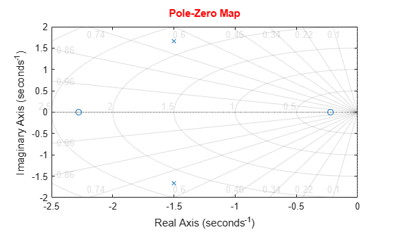
Plot the poles and zeros of the continuous-time system represented by the following transfer function:
sys = tf([2 5 1],[1 3 5]);
pzp = pzplot(sys);
grid on
Turning on the grid displays lines of constant damping ratio (zeta) and lines of constant natural frequency (wn). This system has two real zeros, marked by o on the plot. The system also has a pair of complex poles, marked by x.
Change the color of the plot title.
pzp.Title.Color = [1 0 0];
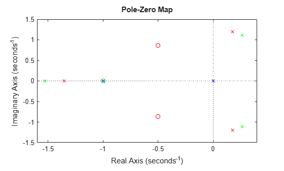
For this example, load a 3-by-1 array of transfer function models.
load('tfArrayMargin.mat','sys');
size(sys)
3x1 array of transfer functions.
Each model has 1 outputs and 1 inputs.
Plot the poles and zeros of the model array. Define the colors for each model. For this example, use red for the first model, green for the second, and blue for the third model in the array.
pzplot(sys(:,:,1),'r',sys(:,:,2),'g',sys(:,:,3),'b');
Plot the poles and zeros of the continuous-time system represented by the following transfer function with a custom option set:
Create the custom option set using pzoptions.
plotoptions = pzoptions;
For this example, specify the grid to be visible.
plotoptions.Grid = 'on';Use the specified options to create a pole-zero map of the transfer function.
h = pzplot(tf([2 5 1],[1 3 5]),plotoptions);
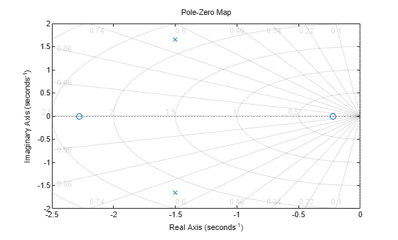
Turning on the grid displays lines of constant damping ratio (zeta) and lines of constant natural frequency (wn). This system has two real zeros, marked by o on the plot. The system also has a pair of complex poles, marked by x.
Input Arguments
Name-Value Arguments
Output Arguments
More About
Version History
Introduced before R2006aSee Also
pzmap | iopzplot | pzoptions | addResponse